Inflationary Cosmology and Cyclic Universe

Contents

Inflation Theory

According to the latest cosmological model, the universe sprang into being about 14 billion years ago. At birth, the space was likely to have been curved and warped due to quantum effect within the tiny speck and time may be meaningless. After about 10-35 seconds, there began a brief period of exponentially fast expansion, known as inflation, that ironed out any curves or warps in space and made the universe flat (because it becomes so large). Inflation also predicts a much smaller initial region, which is required for smoothing out the distribution of matter and radiation, only leaving behind tiny quantum fluctuations that match the observed spatial variations in the cosmic microwave background radiation and provide the seeds for galaxy formation. It also explains the mystery of the absence of magnetic monopole, which had been diluted during the phase of rapid inflation.

Figure 01 Cosmic Inflation

See more in "Theory of Cosmic Inflation".

The orange curve in Figure 01 shows the period of inflation from 10-35 sec to 10-32 sec after the initial expansion. Figure 02 shows the actual size of the universe after the inflation. Our observable unvierse is only part of the whole thing. The mechanism to drive the inflation is related to a "yet-to-be-discovered" inflaton field, which is thought to be similar to the Higgs fields responsible for the mass of the elementary particles. When the temperature fell below a certain value, a phase transition (similar to the transition of water to ice at 0oC with the release of latent heat) of the inflaton field occurred. The phase transition released energy, which was conversed to hot matter and radiation. It also developed repulsive force to drive the inflation. The inflation stopped when the inflaton field settled down into lower energy state.

Figure 02 Unobservable Universe [view large image]

universe. It is hoped that advances in fundamental physics will eventually address these issues. Figure 03a depicts two "energy landscapes" for the process (at a certain point in space). In the old theory, bubbles of true vacuum form by tunneling. It results in a haphazard pattern of bubbles that never merge, so the decay process is never complete leaving an empty universe. In the new theory, the downhill rolling is very slow such that the energy density is almost at a constant value to sustain the exponential expansion. When the field gets to the steeper part of the energy slope, it rolls down faster, and when it finally reaches the minimum, it oscillates and dumps its energy into a hot fireball of particles. At this point we have an enormous, hot, expanding universe, which is also homogeneous and nearly flat - it solves the graceful exit problem on how to stop the inflation sensibly.

Figure 03a Theories of Inflation [view large image]

§ There are at least four different scenarios about the pre-bang universe: 1. Brane collision, 2. Universe inside blackhole, 3. Multiverse, and 4. Tunneling from nothing. (see also the "mathematics of Inflation")

to make it consistent. It is known as the dilaton (~ variable gravitational constant), and can be identified to the vacuum energy density (the dark energy). Thus, this new theory resolves three outstanding paradoxes in one shoot. Such "Inflaton-Higgs-Dilaton" model can be tested by a particular twist in the polarization of the CMBR. The presence of a dilaton field can also be detected by certain gravitational wave imprint on CMBR. This kind of data may be available by 2020.

Figure 03aa Inflation Theory with Higgs

See "The Higgs Bang", and the table on "History of Cosmic Expansion" which shows the closely related events of "inflation" and "origin of matter" (via the appearance of the Higgs boson) in the Electro-weak Era.

Cyclic Universe

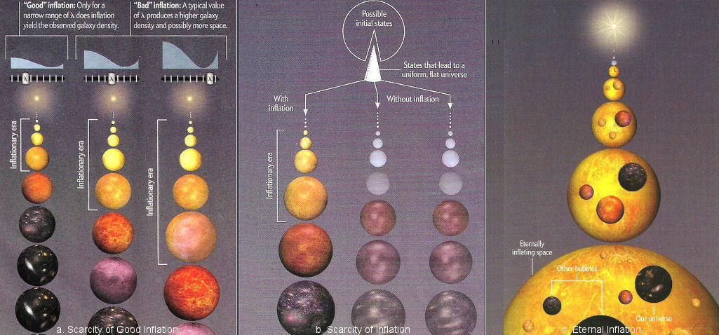In spite of producing predictions in exquisite accord with observations, the theory of inflation is now faulted on theoretical ground. In the April 2011 issue of Scientific American, an article by the theoretical physicist Paul Steinhardt listed three or four shortcomings (as illustrated in Figure 03b) with the theory of inflation and proposed a cyclic universe to resolve the problems. Followings is a summary of his case against the theory of inflation :

Figure 03b Problems with Inflation [view large image]

1. Scarcity of Good Inflation - There are literally an infinite number of models for the theory of inflation. Each of these model is controlled by a parameter called . An inflation model that matches closely with cosmological observations, is restricted to a narrow range around 10^-15 (Diagram a, Figure 03b). Otherwise the model would produce large temperature variation resulting in more stars and galaxies - a more habitable universe - in contrary to the one we live in.



2. Scarcity of Inflation - By extrapolating backward from the current conditions (e.g., flat and smooth) to the initial stage, it is found that only a tiny fraction of the initial states would lead to a uniform, flat universe. A majority of these do not require inflation, and only an infinitesimal fraction would do so by going through a period of inflation. A similar conclusion was reached in the 1980's by Roger Penrose using method in the Kinetic Theory of Gas to arrive at a probability of 1/10¹⁰⁰ for inflation (ends up as flat and smooth universe) to occur (Diagram b, Figure 03b).



3. Eternal Inflation - In the quantum version of inflation, there will be delay in reaching the end point (of inflation) due to quantum fluctuations (in time). If the delay happens to be of a relatively large time interval, the delayed expansion will engulf the well-behaved region, which becomes an island (bubble) surrounded by the (delayed) inflating space as shown in Diagram c, Figure 03b. Such process repeated an infinite times producing an unbounded number of island surrounded by ever more inflating space. In such scenario, all kinds of universes are possible. But if anything that can happen will happen an infinite number of times, then the theory is not a useful tool in generating testable predictions.

In a 2017 Scientific American article, Paul Steinhardt updates his criticism on the theory of inflation :


• Although scale-invariant (similar pattern appears in different scale of the CMBR) can be reproduced by the theory of inflation, such model doesn't seem to be practical.
• No gravitational wave has been detected from CMBR so far.
• The multiverse scenario renders the predictive power of the theory to zero.

The theory of superstring admits up to seven extra spatial dimensions. The cyclic universe model represents our universe as a 3-dimensional brane moving in a 4-dimensional space. It interacts with another 3-dimensional brane via a spring-like force, which is identified with the dark energy. These two branes execute periodic motion as shown in Figure 03c. The moment of collision is perceived by us as the Big Bang. We can never reach out to the extra dimension, only gravity and the dark energy can reside there. Figure 03c depicts the sequence of events during one cycle of the endless oscillations with a more detailed description in the followings:

Figure 03c 3-D Brane Cyclic Universe [view large image]

1. According to the cyclic universe model, the Big Bang is not the beginning of space or time. Instead, it is the moment when gravitational and other forms of energy are transformed into new matter and radiation and a new period of expansion and cooling begins.
2. Hot, dense matter and radiation fills the universe immediately after the bang. The cosmic temperature reaches about 10^{27 o}K. At this temperature, matter exists only in its elementary forms such as quarks, electrons, photons, and the like. However, the temperature remains modest compared to the 10^{32 o}K or higher in the scenario for the usual Big Bang.
3. During the following 9 billion years, the cosmos expands and cools. The elementary constituents clump into protons and neutrons, and eventually atoms, molecules, planet, stars, galaxies, clusters of galaxies, and superclusters. The blueprint had been laid down as tiny density variations (ripples) nearly the end of the previous cycle.
4. Dark energy becomes dominant at this point. The repulsive nature of this substance causes the cosmic expansion to speed up as witnessed by present day astronomers.
5. During the next trillion years, the accelerating expansion will continue and rapidly dilute the universe of the matter content and lumpy structures.
6. The universe is restored to a simple, uniform, and pristine state, which is essentially similar to the prediction by the usual Big Bang theory.
7. However in the cyclic universe model, dark energy is unstable. It will decay near the cycle's end into a form of extremely high-pressure energy that causes the universe to contract slowly.
8. Space becomes increasingly smooth and flat as the contraction proceeds, while quantum effect produces random fluctuations seeding density variations over all the regions.
9. The collision of the two branes produces another moment of Big Bang and starts another cycle.

This model provides answers to two annoying inquiries in cosmology:
1. What went before the pre-big bang, before the pre-pre-big bang, ... ad infinitum -- There could be no beginning or end in a cyclic universe, which may exist forever.
2. What is the 3 dimensional space expands into -- The usual explanation asserts that cosmic expansion is special, it doesn't expand into anything. Since the cyclic universe is a 3-D brane immersing in a 4-D space, the cosmic expansion in this model naturally expands into this 4-D bulk without invoking anything special.

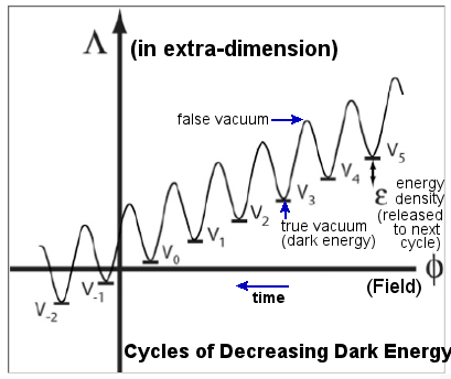		In Paul Steinhardt's version, the 3-D branes are not running in circle repeating themselves endlessly. The evolution is linear as the size of the universe keeps on increasing; it is the contraction of the extra-dimension in the bulk that produces the apparent crunch (Figure 03d). Such scenario solves the problem of low entropy at the beginning of Big Bang. The cosmological constant (dark energy) also evolves along with increasing longevity but decreasing magnitude until it becomes negative to produce the real crunch that ends the cycles (Figure 03e).
Figure 03d Cyclic Universes, New Versiion [view large image]	Figure 03e Constant Cycles	This kind of cosmological model suffers the apparent fault that it is based on an un-proven theory. It is viable only if superstring passes some tests successfully

A Simple Mathematical Model

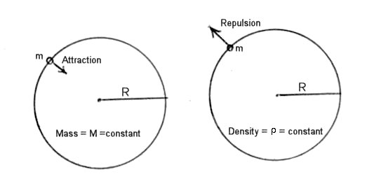The concept of cosmic inflation can be illustrated by simple mathematics using only elementary calculus. Suppose the universe is uniform and isotropic as demonstrated by observations. This means that every point in the universe is similar to every other point and can be considered as the "centre" (Figure 04). Now consider a "test particle" of mass m and at distance R from the centre. Since only mass inside the sphere has a net effect on the particle, and if the total mass M insider the sphere of radius R is constant, then the potential energy of the particle is:

Figure 04 Repulsion vs Attraction [view large image]

Thus in this scenario, there is a repulsive force to drive the inflation (Eqs.(4) and (5)); matter and radiation are being created according to Eq.(6). Under normal circumstance, the matter density would decrease with the expansion. It is thought that the decay of the "inflaton field" to the lower energy state is responsible for keeping the matter density constant. Figure 05 shows the variation of the energy density since the Big Bang. It maintained a constant value during the inflationary era as

Figure 05 Energy Density [view large image]

described in the simple mathematical model. The energy density of water (1021 ergs/cm3) and of an atomic nucleus (1036 ergs/cm3) are included in the graph for comparison. A mathematical treatment based on general relativity can be found in the appendix on "Relativity".

Cosmic Evolution of Entropy

		Entropy is defined as the degree of randomness§, which can be expressed alternatively as the degree of freedom in a system (the degree of freedom is the number of different parameters or arrangements needed to specify completely the state of a particle or system). The evolution of entropy in the universe as a whole can be separated into four phases as described briefly below (also see Figure 06, which supplies more details):
Figure 06 Evolution of Entropy [view large image]	Figure 07 Initial Entropy [view large image]

1. The inflaton field is a coherent system changing rapidly until the end of the inflationary era. Such system has very few degrees of freedom, so it has a very low entropy. (Figure 07, it also shows a brief portray of leptogenesis, which is a theory to explain the asymmetry between matter and anti-matter.)


2. At the end of inflation the energy density of the inflaton field decays to zero (see Figure 03a), thereby releasing lots of energy to produce particle anti-particle pairs, and to heat up the universe. It is this "reheating" that produce lots of degree of freedom, and thus lots of entropy.


3. The infusion of energy dU ceased once the inflaton energy density vanished, i.e., dU = 0. According to the thermodynamics relation dU = TdS - pdV (where p = pressure, V = volume, T = temperature), the entropy now varies as dS = (p/T)dV. The universe was dominated by radiation up to 10⁴ years after the Big Bang. During this era p T⁴; since in term of the size of the universe R, T 1/R, dV R²dR, thus dS dR/R and the entropy S log (R).


4. In a matter dominated universe p = 0, thus dS = 0; the entropy is conserved as a whole for the rest of the cosmic expansion.


5. If acceleration of the cosmic expansion is taken into account, then there is infusion of energy by an amount dU. The entropy dS dU/T will increase until space is nearly empty in attaining the highest entropy state.

The scenario above assumes a quasi-equilibrium approach, which is not entirely correct with the cosmos expanding rapidly. Diagram (a) in Figure 08 is a more realistic sequence according to Boltzmann's general definition of entropy in which the evolution of entropy is described by the phase point moving in phase space without any assumption concerning the equilibrium of the system. Diagram (b) shows another sequence of entropy evolution when the gravitational degrees of freedom is introduced to the system.

Figure 08 Entropy and Gravity [view large image]

It is pointed out that the above model fails to explain what set up the initial low entropy state. An alternate scenario adds a period of prehistory (see Figure 09) in which space was nearly empty (thus avoiding the necessity of setting up the low entropy state), and inflation was brought about by fluctuation of quantum fields. It implies the existence of multiverse where the arrow of time may run backward. The appearance of stars and galaxies is a temporary deviation from the equilibrium of empty space.

Figure 09 Entropy Evolution with Prehistory [view large image]

Magnetic Monopoles

Near the center ( about 10-29 cm ) there is a GUT symmetric vacuum. At about 10-16 cm, its content is the electroweak gauge fields of the standard model. At 10-15 cm, it is made up of photons and gluons. At the edge to the distance of 10-13 cm, there are fermion-antifermion pairs. Far beyond nuclear distances it behaves as a magnetically-charged pole of the Dirac type. In effect, the sequence of events during the earliest moment of the universe had been fossilized inside the magnetic monopole.

Figure 10 Monopole Structure in GUT [view large image]

In this theory, the monopole is portrayed as a soliton which is stable - cannot decay to lower mass particles. In effect, it closes the loophole for explaining its absence in nature, and prompts the invention of "cosmic Inflation" to explain away the problem by dilution. GUT also fails in its prediction of "proton decay".

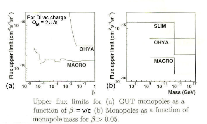Figure 11 shows the flux upper limit of monopole search in cosmic ray. It indicates that the detectors are sensitive only up to that level and failed to detect any monopole; in fact the flux could be even lower all the way down to zero. The data are in unit of cm-2s-1sr-1 (sr = steradian, is the SI unit of solid angle). The flux upper limit is in the range of 10-15 - 10-16 with this unit. Such flux level is much lower than that for the cosmic ray bombarding the Earth regularly in the range of 1 - 10. The MACRO experiment comprised three different types of detector : liquid scintillator, limited stream tubes, and NTDs (Nuclear Track Detector for detecting cosmic ray tracks inside solid material). The OHYA experiment (using array of

Figure 11 Monopole Flux Upper Limit [view large image]

NTDs) is located inside a mine in Japan. SLIM is a high-altitude experiment.