Home Page Overview Site Map Index Appendix Illustration About Contact Update FAQ


Superclusters


Large Scale Structures, Simulation

Contents

Numerical Evaluation with Moving Mesh
Moving Mesh Application to Cosmic Hydrodynamics
Results of the Simulation

  • Numerical Evaluation with Moving Mesh

    In numerical evaluation of functions and differential equations the independent variables are digitalized by adding infinitesimal steps one after another in constant amount as shown in Figure 03-05b. The most convenient choice is to divide the range into N partitions, i.e.,
    x = (xN - x0)/N (Figure 03-05b,a). However, there are cases when other choice such as equi-distribution of some attribute is more suitable. Such choice would alter the size and boundary of the physical meshes x, and y as shown in Figure 03-05a for 2-D case.
    Moving-Mesh, Concept Moving-Mesh, Example 
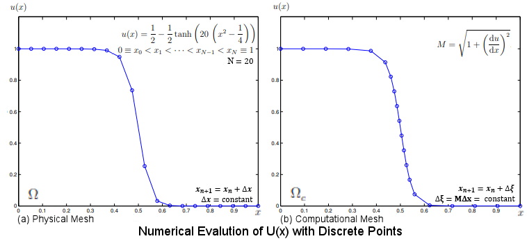
It is thus called the method of moving mesh. For example, the step can be chosen as constant arc-length Mx (see Figure 03-05b,b). The arc M is called the monitor function transforming the physical mesh
    x to the computational mesh . The new choice derives more points in the range with steeper descent, and thus improves the numerical approximation.

    Figure 03-05a Moving Mesh, Concept

    Figure 03-05b Moving Mesh, Example [view large image]

    For the case of horizontal straight line u = constant, du/dx = 0 giving M = 1 and = x.

  • See "A Moving Mesh Finite Element Method for the Numerical Solution of Partial Differential Equations and Systems" for detail.

  • Moving Mesh Application to Cosmic Hydrodynamics

    In application of the moving mesh method to cosmic hydrodynamics, the meshes are constructed in the form of Voronoi tessellation (some sort of mosaic as shown in Figure 03-05c) where the movement of the edges are determined by the net velocity w = (wL+wR)/2 between 2 meshes (the insert in Figure 03-05c shows the rough idea, see full detail in "Galilean-invariant Cosmological Hydrodynamical Simulations on a Moving Mesh"). A computer simulation of the large scale structure using such method was unveiled in May 2014.
    Moving-Mesh Moving-Mesh Evolutiob It has successfully reproduced many observations from clusters of the galaxies to the types of galaxies. The simulation involves solving the equations of gravity and hydrodynamics as functions of time. Resolution of the cosmic structure depends on the size of the mesh, nothing smaller than such size will show up in the simulation. Starting from the initial conditions for the angular velocity v
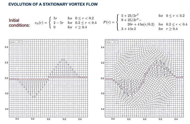
(r) and pressure P(r), Figure 03-05d portrays the evolution of the meshes for v
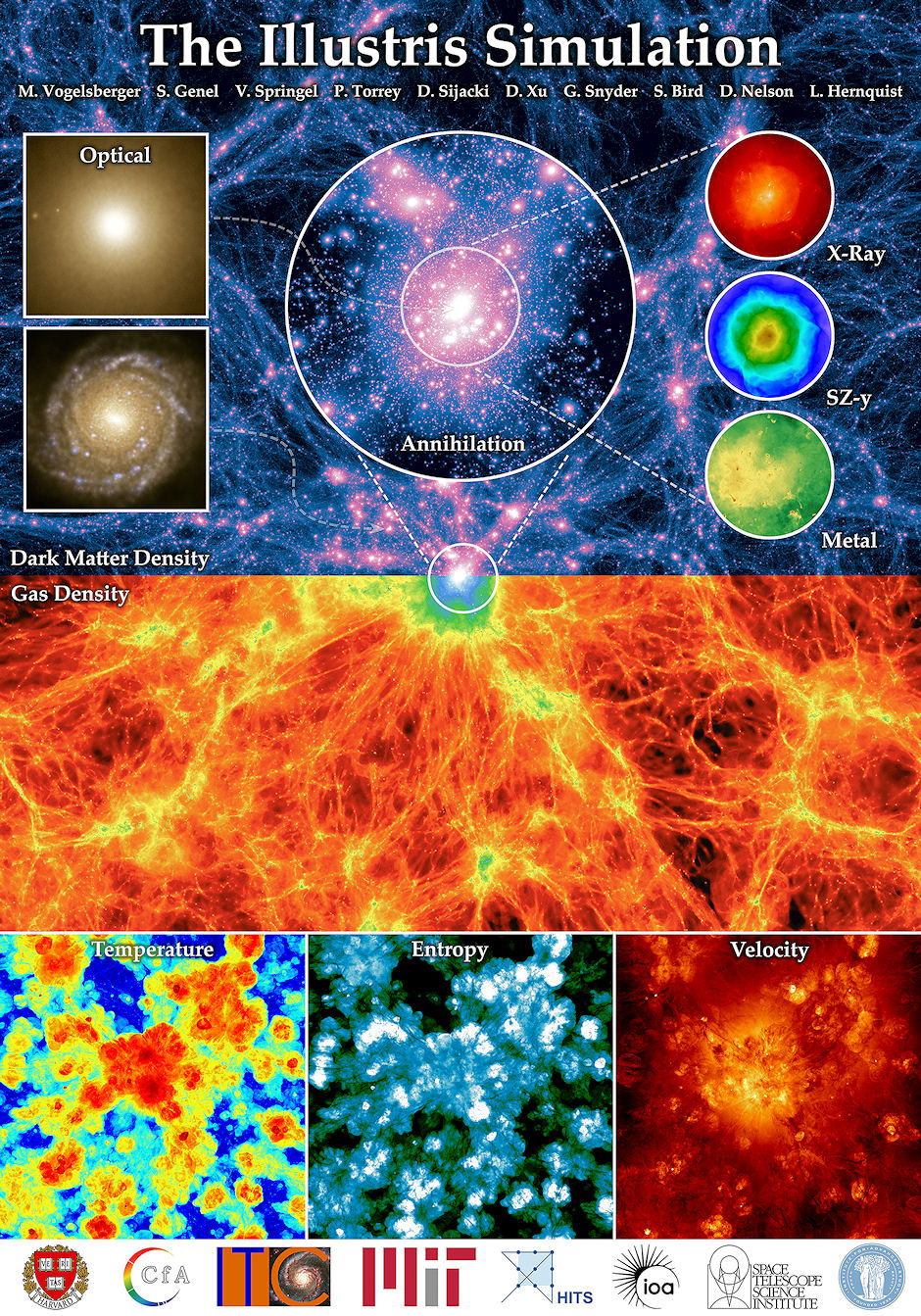
(r) some moment later. It shows that the meshes are changing shape and moving in the direction of the velocity field.

    Figure 03-05c Moving-Mesh Construction


    Figure 03-05d Moving-Mesh Evolution [view large image]


  • Results of the Simulation

    Illustris Large Scale Evolutiob The cosmic model is called Illustris (see logo in Figure 03-05e). It traces the evolution of both visible and dark matter starting just 12 million years after the Big Bang. It ends up at the present epoch showing the large structure in clusters of galaxies as well as smaller details in individual galaxies. The simulation contains 12 billion cells in a cube of (106.5 Mpc)3 across the universe. The smallest size scale over which the hydrodynamics is resolved, is 48 pc (about the distance from the Sun to its nearer neighbour stars). It took about 16 million CPU hours on stat-of-the-art desktop computers to complete the simulation. Some of the results are shown pictorially in Figure 03-05f. Many of the simulated features are summarized in Table 03-01. The work is published in the 8 May 2014 issue of Nature ("See origin article "Properties of Galaxies Reproduced by a Hydrodynamic Simulation").

    Figure 03-05e Illustris Logo [view large image]

    Figure 03-05f Large Scale Evolution [view large image]

      The input parameters are (see cosmological constants) :
    1. matter density m = 0.2726,
    2. dark energy density = 0.7274,
    3. baryon density b = 0.0456,
    4. Hubble expansion rate H0 = 100h km/s-Mpc, h = 0.704 for the present epoch,
    5. spectral index of the primordial power spectrum ns = 0.963,
    6. root mean squared amplitude of mass fluctuations in 8h-1 Mpc spheres s = 0.809,
    Initial Conditions : at z = 127 in a periodic box with a side length of about 106.5 Mpc and gas temperature 245 K.

    Cosmic Feature System Scale Simulation Observation
    Cluster of Galaxies ~ 100 Mpc Super-clusters in the form of Cosmic Web Same
    Intergalactic HI Clouds ~ 10 Mpc Number of absorbers as function of column density In good agreement
    Cluster Satellites ~ 200 kpc Number of satellites from halo center In good agreement
    HI Gas in Galaxy ~ 50 kpc Mass of HI gas as function of galactic mass Discrepancy in elliptical galaxies
    Metal Content in Galaxy ~ 50 kpc Metal content as function of galactic mass In good agreement
    Galaxies Morphology ~ 50 kpc Mixture of elliptical, spiral, irregular galaxies In good agreement
    Low-mass Galaxies < 1010 Msun ~ 5 kpc Build up too early ~ 3 times later in observation

    Table 03-01 Features in Cosmic Simulation (click underlined text to see pictorial illustration)

    The large scale features in the table are the result of processes within size scale of a few tens pc from gas cooling; stellar evolution; supernova explosion; chemical elements creation; AGN feedback; supermassive black holes formation and accretion.

    The simulation demonstrates that the current knowledge on the large cosmic structures is essentially correct. It offers a tool to cross examine observation and theory in future development.

    Go to Next Section
     or to Top of Page to Select
     or to Main Menu

    .