Home Page Overview Site Map Index Appendix Illustration About Contact Update FAQ


Mathematical Minimum (for Aspiring Physicists)


Contour Integrals

Complex Number It was known in the 17th century that the roots of polynomial equations, i.e., when f(x) = 0 in:
f(x) = anxn + an-1xn-1 + +a1x + a0 (such as f(x) = x2 + 2 = 0 at x = ),
often involve square roots of negative numbers. It was realized subsequently that the complex number, which is defined as the combination of a real number and a square root of negative number, is more useful than the real number alone. In the Cartesian form the complex number z is expressed as z = x + iy, where the negative sign in the square root has been absorbed into the symbol i = . In terms of the polar coordinates r and , z = r ei, where r2 = x2 + y2, and tan = y/x (Figure 08). The complex conjugate of z is defined as z* = x - iy or z* = r e-i, such that z z* = r2. The term "imaginary" for the part associated with "i" was coined by
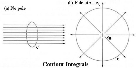
Figure 08 Complex Number [view large image]

René Descartes and was meant to be derogatory. The study of functions of a complex variable is known as complex analysis. Unlike real functions, which are commonly represented as two-dimensional graphs, complex functions have four-dimensional graphs.
Contour Integral Contour integral is related to a special class of complex function called analytic function denoted here by f(z) = u + iv, with the complex variable z = x + iy. It has the property that the derivative df(z)/dz exists uniquely at every point. In other words, the way z 0 is indepen-dent of the path, e.g., we may choose a path with x=0 or y=0. It follows that the real and imaginary parts of an analytic function are solutions of the two-dimensional Laplace equation:

Figure 09 Contour Integral [view large image]

, .
It can be shown that the contour integral of an analytic function f(z) around any closed path c is zero, i.e.,
---------- (18)
This is illustrated in diagram (a) of Figure 09. The vanishing integral is related to the fact that the number of lines entering and leaving the contour are the same. In case there is a source or sink (collectively called a pole) within the region so that the number of lines entering and leaving the contour is not balanced as illustrated in diagram (b) of Figure 09, the contour integral becomes:
---------- (20)
where z0 denotes the position of the pole. For example,
---------- (21)
In general, for a function with multi-poles such as f(z) / (z-z1)(z-z2)...(z-zn), where f(z) is an analytic function, the contour integral enclosing all these poles is given by 2i [f(z1)/(z1-z2)...(z1-zn) + f(z2)/(z2-z1)...(z2-zn) + ... + f(zn)/(zn-z1)(zn-z2)...].

A technique to evaluate ordinary integration is to use the contour integral with poles whenever Eq.(17) is satisfied. For example, considering the following integral:
Contour I = 
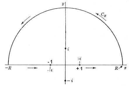
dx / (x2 + 1) ---------- (22).

This integral is part of a closed contour integral, which has a pole at z = i (see Figure 10):

Ic = dx / (x2 + 1) + cR dz / (z2 + 1) = I = 2i [1/(z + i)]z=i = 2i (1/2i) = ------------ (23),

Figure 10 A Contour Loop
[view large image]

where the second term vanishes if we let the radius of the semi-circle R .


Another neat trick is to create pole(s) inside the loop (contour). Considering the following integral:

I = dx / (1 - x2) ---------- (24)

There are two poles at x = +1 and x = -1, right on the real axis. In order to apply the loop in Figure 10 to evaluate this integral we can artificially move one of the poles a wee bit up and the other one down by an amount i as shown in Figure 10, and then let 0 at the end. Thus,

Ic = dx / (1 - x2) + cR dz / (1 - z2) = I = 2i {[1/(1+z)]z=1+i}0 = 2i (1/2) = i ---------- (25).

Actually, the answer can be obtained as easily by substituting y2 = -x2, dx = i dy in Eq.(24), and using the result from Eq.(23).

Go to Next Section
 or to Top of Page to Select
 or to Main Menu

.