| Home Page | Overview | Site Map | Index | Appendix | Illustration | About | Contact | Update | FAQ |
 |
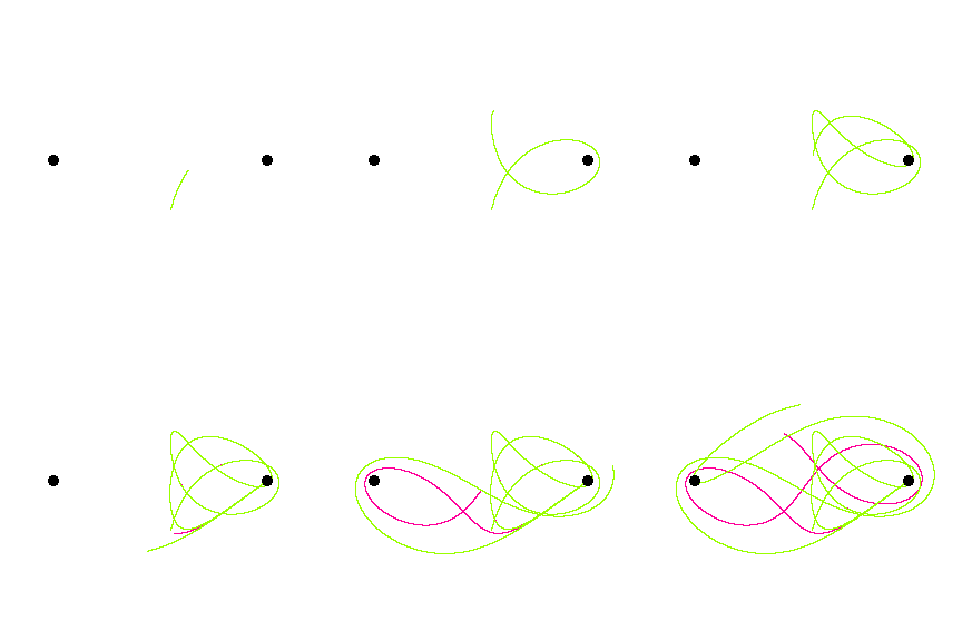
At the end of the 19th century, the French mathematician Henri Poincare tried to solve the differential equations for the three body problem. It was noticed that the orbit is not periodical anymore (in contrary to the case with just two body), actually the motion appears to be random. Then it was found that the solution is "exquisite sensitivity to initial conditions". The object would follow a very different path at the slightest change of initial condition. Figure 01 is an animation showing two paths of a third body under the gravitational influence of two massive objects. The paths start at the same position but the velocities differ by 1%. Initially the paths are very close, the difference becomes apparent after a while. Sixty years later, this kind of divergent behavior was re-visited by a meteorologist, named Edward Lorenz (1917-2008), with a set of 12 equations used to model the weather. He found the system evolves differently |
Figure 01 Chaos |
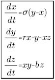
by just a very slight variation of the initial condition. This divergent behavior is now known as the butterfly effect - the slightest disturbance of the air by a butterfly would cause a global weather change a year later. Eventually, Lorenz simplified the number of equations to three, |
 |
 |
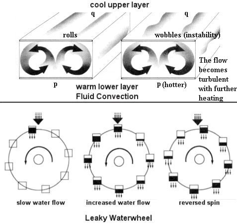
and the system still exhibits the same kind of divergent behavior. The simplified system simulates the dynamical behavior of convection rolls in fluid layers that are heated from below (Figure 02). This is a crude approxi-mation of the air circulation at different latitude of the Earth (Figure 09-10) It is also applicable to a leaky waterwheel (Figure 02). A waterwheel built from cups with equal sized holes in the bottom of each cup is allowed to turn freely under the force of a steady stream of water poured into the top cup. The waterwheel turns smoothly if the water pours down slowly. But as the water flow is increased, the wheel tunrs faster, the buckets have little time |
Figure 02 Lorenz Systems |
Figure 03 Lorenz Eqs. |
to fill up or become empty. The system changes to chaotic, and the spin will slow down or even reverse. It never repeats itself in any predictable patterns under these conditions. Figure 03 displays the Lorenz equations, |
 , r, b are the parameters;
 : Prandtl number = (fluid viscosity/thermal conductivity),
 = 10, r = 28, and b = 8/3, the system shows chaotic behavior. The variation of x, y, and z with time is displayed in Figure 04, which shows oscillations between some limits - it is not exactly the same as the white noise. There is a certain ordered patterns, it seems to be disorderly because the patterns are not readily appreciable.
The behavior is easier to visualize
 |
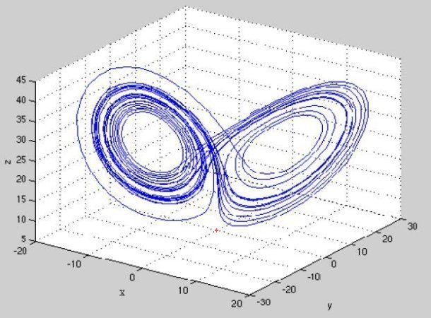 |
if the development of the system is plotted in the phase space, where the values of x, y, z define each point in the graph. It is then clear that the system is confined to a certain region, namely the two shells (see Figure 05). However, the time progression of the points is not obvious. It either relies on color codes (for example, blue for earlier and red for later moment) or animation (which shows the points spreading from a small initial region) to display the evolution of the |
Figure 04 Time Series [view large image] |
Figure 05 Phase Space [view large image] |
system. The region occupied by the system in the phase state, namely the butterfly or the shells, is known as Lorenz attractor, to which the dynamical motion will always converge no matter how far off initially. |
 |
 |
 |
The solutions of the Lorenz equations also depend on the parameters. When r is small, e.g., r = 10 all solutions tend to a fixed point as shown in Figure 06; this is not chaos. Starting from r ~ 14 the fixed points lose their stability. For r = 21, the system begins to exhibit transient chaos. This means that although it begins as a chaotic process, its long- |
Figure 06 r = 10 |
Figure 07 r = 21 |
Figure 08 r = 400 [view large image] |
term behavior becomes periodic (see Figure 07). The critical value for r that is required to produce chaos is r > 24 (Figure 04). However, for very large value of r such as r = 400, all solutions become periodical again (see Figure 08). |
 ]2} / dt = - {
 x2(t) + y2(t) + [z(t) - (r +
  )/2]2} + b [(r +
  )/2]2
)/2]2 ]2} / 2. The rate of change as indicated on the right hand side is negative for large value of (x,y,z). It means that the path spirals inward when it is far away from the origin. For small value of (x,y,z) the rate of change is positive (for b > 1), which means moving outward. Thus, points on the orbit outside the Lorenz attractor (in the shape of an "8") always return to the compact region and hence the name.
 |
The period doublings come faster and faster, until we have passed infinitely many of them. Still for a finite R, but the behavior becomes "chaos" meaning a small difference in the initial condition will diverge to two completely different pattern.
|
Figure 09 Logistic Equation |
logistic solution by specifying the value of R, the initial population, and the number of iterations. Figure 09 is the results of six runs obtained from there with initial population = 0.1, and 80 generations. |
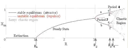 |
Figure 10 summarizes the variation of the population with the changing values of R. Xm represents either the steady or stationary value of X. The initial bifurcation point occurs at R1 when the population can sustain itself in a steady state at a stable value of Xm. The next bifuraction point R2 introduces oscillation between two stationary points a and b (Figure 09c). The "period four" (R3) solution shows four stationary points |
Figure 10 Bifurcation |
c, d, e, and f (Figure 09d). Higher value of R, e.g., R4 produces so many stationary points, it is very difficult to follow the details (Figure 09e) in such chaotic region. |
 i = (Ri - Ri-1) / (Ri+1 - Ri)
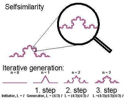 |
The Koch curve has been constructed according to the idea of self-similarity. It starts from a straight line. Then add an equilateral triangle to the middle third of each side. A Kock curve is obtained by repeating the procedure on each successive (and shorter) straight line (see Figure 11). It is noticed the area enclosed within does not increase with the length of the lines as prescribed by the Euclidian geometry. To get around this difficulty, mathematicians invented fractal (fractional) dimensions. The fractal dimension of the Kock curve is somewhere around 1.26. Now fractal has come to mean any image that displays the attribute of self-similarity. It exposes the abstract geometrical nature of chaos. |
Figure 11 Koch Curve |
 . In other word the length L depends on the size of measuring stick, which becomes smaller and smaller with increasing value of n.
 |
|
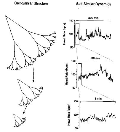
Figure 12 Fractal in Real-World [view large image] |
 |
Starting with an initial value z(0) equal to the coordinates of each point of the complex plane (imaginary axis in the vertical, real axis in the horizontal), the function diverges (the value of z' moves more and more away from the initial value) for many of such points. On the other hand, for some points, the result remains definitively within a limited interval : the function does not diverge, even for an infinite number of iterations. The points for which the function does not diverge give a set called connected Julia set (diagram a, Figure 13). In some cases a Julia set is fragmented (disconnected) as shown in diagram b. If, instead of giving c a fixed and arbitrary value, we give for any point of the complex plane an initial value c = z(0), we obtain a more complex mathematical object called the M (Mandelbrot) set (the black part at the center of diagram c). The points for which the values of z diverge do not belong to the filled-in Julia set: they are situated outside. But one can obtain extra information by giving them a brightness or a colour that is |
Figure 13 Julia and M Sets [view large image] |
a function of the number of necessary iterations to observe the divergence. In other words this colour is a measure of the speed at which the function diverges for this point. |
 |
those fluctuations become too great for the open system to damp, the system will then departs far from equilibrium and be forced to reorganize. Such reorganization generates a kind of "dynamic steady state" provided the energy flow rate exceeds the thermal relaxation rate. The feedback loops are positive in this kind of process. Complexity itself consequently creates the condition for greater instability, which in turn provides an opportunity for greater reordering.
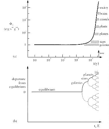
Another approach to view the development of complexity is through the concept of energy flow per unit mass. Figure 14(a) shows the increase of complexity as the energy flow (per unit mass) into the various systems increases over the age of the universe. Figure 14b depicts qualitatively the departure from equilibrium at each bifurcate point where the energy flow has reached a critical value and thus can promote more complexity in the system. The dotted curves indicate the options that have not been taken by the evolution. The bifurcation is created when the system enters a nonlinear mode beyond |
Figure 14 Complexity and Energy Flow [view large image] |
some energy threshold. Thus the development of complexity is a phenomenon closely related to the chaos theory or nonlinearity with a positive feedback loop. |