Thermodynamics

Non-equilibrium Thermodynamics & Life (2020)

Equilibrium Thermodynamics + Irreversibility

There are two different physical properties of materials in thermodynamic system :

• Intensive Property - it is a bulk property that does not depend on size or the amount of material. Examples include the density , temperature T, pressure P, chemical potential , ... In equilibrium thermodynamics, the intensive properties are homogeneous, isotopic, and unchange through out the system. Such requirements are identified as :
  
  • Thermal Equilibrium - the temperature T is uniform through out the system (Figure 01,a).
  • Mechanical Equilibrium - the pressure P is balanced by the external forces (Figure 01,b)
  • Chemical Equilibrium - the chemical potentials for the various species remain constant, i.e., absence of any chemical reaction (Figure 01,c).

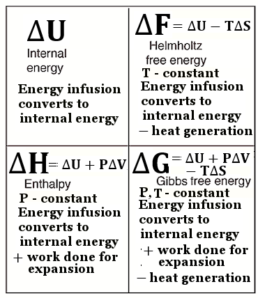
  Extensive Property - such as the internal energy U, volume V, entropy S, and number of particles N in the system. They can be added to or removed from the system. In thermodynamic equilibrium, some of the extensive properties such as the Gibbs Free Energy and entropy have to be at its minimum or maximum respectively as shown in Figure 01,d. As all these variables are held fixed at equilibrium, for example, the internal energy U can be expressed as : U = TS - PV + N ----- (1).

  Figure 01 Equilibrium Thermodynamics, Conditions

  Such formulation with everything unchanged is not very useful in describing the changing world. Equilibrium thermodynamics gets around this problem by considering only the initial and final equilibrium states without regard to the intermediate details.

		Step 1 - the adiabatic process is the compression stroke that runs so rapidly allowing no change of heat Q, i.e., Q = 0. Figures 03 and 02,a show that the temperature T increases by certain amount during the process according to the ideal gas law PV = NkT. Step 2 - this combustion phase introduces heat into the system. It also runs so rapidly that the temperature has no chance to be altered, i.e., T = 0 - an isothermal process.
Figure 02 Equilibrium Thermodynamics, Carnot Cycle [view large image]	Figure 03 Processes	Step 3 - it is the step 1 in reverse as the heat produces work to expand the volume and to reduce the temperature. Step 4 - the exhaust stroke removes the residual heat to prepare for the run of the next cycle.

Figure 02,b shows the same cycle in the real world. The principle is the same, except the difference in detail making it irreversible.

The second law of thermodynamics links the universal increase in entropy to the irreversible process such as the one shown in Figure 02a going from state I to II. In general, the transition matrix element for the backward process

(III) ~ (III) exp(-S/kB) ----- (2a), where S = (SQ = Q/T) entropy released to heat bath + (SII - SI) for internal change of state. Such entropy dissipation is a very important process in non-equilibrium thermodynamics. Some microscopic processes are reversible (at least in theory), i.e, S = 0; however S >> kB for almost all macroscopic processes, so that (III) ~ 0, it is virtually impossible to run the process in reverse and used as an arrow of time (Figure 02b).

Figure 02a Irreversibility

(Figure 02b)    (Figure 02c)

Figure 02c is a misleading example of reversible process in daily life. The re-solidifying chocolate cannot be a reversible process as it would never return to the original shape by itself.

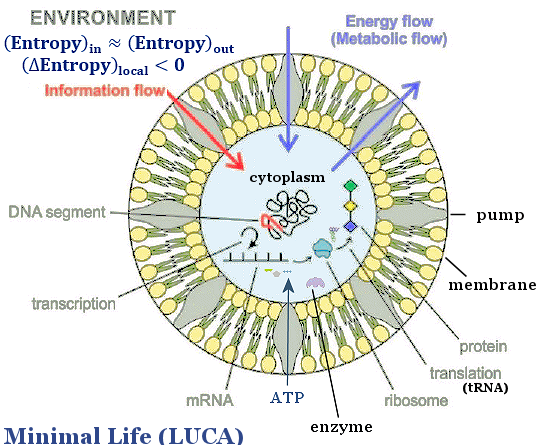
NB : Since the condition for applicability of Eq.(2a) is S = S_Q + (S_II - S_I) 0, there would be entropy dissipation even when S_Q = 0. In such case, the source comes from a lower entropy state descending to a higher one, i.e., (S_II - S_I) > 0, and it is supposed to occur spontaneously. However, for S_Q 0, (S_II - S_I) can be negative (driven by free energy infusion) as long as the inequality is satisfied. It means that orderly product can be created out of irreversible process at the expense of generating dissipative entropy S_Q . The environment serves as the heat bath (heat sink).

		It is this kind of irreversible process we will refer to subsequently for generating orderly structures (See Figure 02d). The simple mathematical formula of Eq.(2a) becomes increasingly un-sustainable in many far from equilibrium processes. However, it is still applicable in principle to the generation of locally ordered structure as demonstrated by the biological process in real life (Figure 02d).
Figure 02d Processes in Life [view large image]	Figure 02e Free Energy	In that illustration, "Free Energy" is defined as the kind of useful energy which can run a process (to do work). Figure 02e summarizes the conversion of the infusing energy to various kinds of Free Energy under different condition.

BTW, k_B = 1.38x10^-16 erg/K^o is the Boltzmann constant. It has the dimension of entropy.

Local Equilibrium Thermodynamics

		In Local Equilibrium Thermodynamics, the whole system is not in equilibrium; but the intensive variables such as T, P, ... can be defined within a small volume, i.e., they are homogeneous (well-mixed) inside that volume (Figure 04,a). In addition, if the system can be described by mathematical formulas, then these intensive variables have to be differentiable, i.e., the functions should be smooth, continuous, and no break, angle, or cusp so that the derivative exists across the
Figure 04 Local Equilibrium Thermodynamics	Figure 05 Diffusion [view large image]	whole system (Figure 04,b). Accordingly, the so-called Gibbs equation in the form of Eq.2 can be carried over with the difference "" replaced by the differential "d" (see Figure 04,b) : dU = TdS - PdV + dN ----- (3).

A few comments :

• For monotonous decreasing n(x) (from the origin of high concentration) the second derivative in Eq.(6) is negative, while
  ~ (kT)log_e(n/n₀) is also negative for (n/n₀) < 1 (n₀ is the initial density). In such case, the entropy density s(x) always increases.
• At t = 0, the initial density n₀ spreads uniformly at a region up to x₀ within which (n/x) 0, the entropy density s is a constant.
• As t , the whole system is at equilibrium n/x 0, so that s/t = 0 indicating no more change in entropy (see Figure 05).

0 ----- (9),

Steady State

A Rayleigh-Bénard (R-B) system is created by heating a thin film of viscous liquid (oil, for example) from the bottom. For certain threshold of heat infusion, convective cells of regular form appear in the system (Figure 06,a). The formation arises via the upwardly buoyant force against the opposing viscous resistance as shown mathematically by the equation of motion in fluid dynamics (see Figure 06,b for configuration and pattern of convective flow).

Figure 06 Rayleigh-Benard Convection [view large image]

Characteristic of the R-B system can be discerned from the value of the dimensionless Rayleigh number Ra :


• For Ra < 1708, the system is governed by heat conduction, there is no movement of the fluid (Figure 07,a).

At Ra = 1708, convective flow commences. For a system with all the physical parameters fixed, Ra is determined solely the the temperature difference (Tb - Ts). For Ra = (4000 - 10000) the flow becomes increasingly unstable as shown in Figure 07,b,c. Beyond this range, the convection becomes too complex to form any regular pattern. Depending on the boundary at the top, the temperature Ts is constant as shown in Figure 07 (for most numerical simulations), or it varies from hotter at the center of the hexagonal to colder at its edge as shown in Figure 06,b (in experimental study).

Figure 07 Temperature Variation with Ra [view large image]

In general, steady heating at the bottom will develop a regular pattern for the velocity field (Figure 06,b) as the heat is dissipated at the top. This is an example of dissipative structure which will collapse once the supply of energy is removed.

Updated 2021.


Here's an astronomical example of the polygonal surface patterns on Pluto. A research in 2021 suggests that they form by sublimation-driven convection as the surface cooling by nitrogen-ice dominates over the heat flux at the bottom of the layer due to radiogenic heating in the rocky core and secular cooling/heating of the interior. See "Sublimation-driven convection in Sputnik Planitia on Pluto" and a video (Figure 07b). Anyway, the patterns would form as long as heat is dissipated from the surface.

Figure 07b Pluto, Polygon

End of 2021 Update.

There are 2 ways to calculate the entropy production in the system :


1. The variation of entropy S = S_p - S_E, where S_E is the total entropy infusion from the external environment, while S_p is the total entropy generating within the system. For steady state S = 0, and thus,
   S_p = S_E = dQ/T ----- (14),
   where the heat flow to the system dQ is the difference between the inflow from the heating surface and the outflow to the inner surface of the container (in contact with the liquid). The integration is over the entire surface and duration.
   
   The conductive heat transfer is : dQ/dAdt = -k(T_q - T)/x, where A is the cross-section area, t the time, x the thickness of the conducting plate, T_q the temperature of the heat source, and k the conductivity in erg/cm-sec-K^o.


2. Another method is to adopt the formula in Eq.(8) for local equilibrium thermodynamics.

It turns out that the 2 methods to calculate entropy production are essentially in agreement for wide range of Ra (Figure 09,b) except: When the experiment (numerically in Figure 09) turns on initially, there is substantial difference until the system stabilizes to steady flow. The effect is attributed to the assumption of local equilibrium in computing Sg. Such assumption is not valid in a complex, unsteady state (see Figure 09,a).

Figure 08 Entropy Spatial Distribution, Ra = 20100 [view large image]

Figure 08 shows the entropy spatial distribution from two-vortex numerical simulation with Ra = 20100. The minima occur at the locations of the vertexes, i.e., there's more orderly formation at those spots.

	Figure 09,b shows increasing entropy production as the value of Ra goes up. The insert displays the entropy production difference (Sp - Sg), which increases with Ra. The effect is also attributed to the inadequate assumption of local equilibrium.
Figure 09 Benard Cell Entropy Production [view large image]	See "The Character of Entropy Production in Rayleigh–Bénard Convection".

Dissipative Processes, Structures and Life

The various steps of dissipative process is depicted in Figure 02d. The portion starting from equilibrium to lower entropy is in general for both animate and inanimate systems, while the latter half concerns mostly with living entities. Here's the first half :


• When a system of particles or anything leaves to its own devices, it tends to arrive at an equilibrium configuration doing nothing. This is the state at maximum entropy as envisioned by Boltzmann back in 1872.


• Things start to get interesting with injection of free energy from outside, it turns from an isolated to open system.

  (a) Perturbation - Initially, the infusing energy may not be enough to un-settle the system. In some circumstance, it can run in a positive feedback loop such as the simple example : x(n+1) = 1 + x(n) , where x(n) stands for a variable with time step (or generation, ...) "n". Starting from x(0) = 1, it could attain a very large value as n increases. Usually, the unrestrained growth is modified by a negative feedback loop or cutoff at a special point.

  Figure 10 Free Energy [view large image]

  (b) Instability - In our case, x(n) could be the infusing energy building up at some location. The accumulation terminates when it reaches the point of instability. (c) Irreversible process - It starts to run at that point. The system evolves and finally settles down to a stable state with lower entropy. (see irreversibility).

• Figure 11,a shows the increase of structural complexity as the energy flow (per unit mass) into the various systems increases over the age of the universe.
  Figure 11,b depicts qualitatively the departure from equilibrium at each bifurcate point where the energy flow has reached a critical value and thus can promote more complexity in the system. The dotted curves indicate the options that have not been taken by the evolution. The bifurcation is created when the system enters a nonlinear mode beyond some energy threshold. Thus the development of complexity is a phenomenon closely related to the chaos theory or nonlinearity with a positive feedback loop.
  
  
• During the period of re-organization, the various components in the system interact according to the principle of least resistance (Figure 12c), which endows the ability to self-assemble or self-organize into complex structures and to self-maintain in space and time, i.e., reaching a steady state, far from thermodynamic equilibrium and with lower entropy at some spatial location.



		At steady state, the total entropy entering from outside is balanced by the total entropy removed from within. However, as shown in the example of Rayleigh-Benard convection, entropy can be lower than the average at some spatial location, that's where orderly structures are created. As shown in Figure12,b, the
Figure 11 Dissipative Structures [view large image]	Figure 12 Dissipative Process, Part 1	entropy dissipation into space SQ = Q/T can be enormous since the temperature T is very low in outer space - a factor favorable for the existence of life.

System	Source	m Energy Flow (erg/s-g)	Comments
First Galaxy	GM/R	1.5	M = 1012Msun, R = 10 kpc, contraction time ~ 300 My
Sun (ongoing)	Solar Constant	2	m = (Solar constant) x (4D2/Msun), D = 1 AU
Earth	GM/R	200	Accretion time of planetesimals ~ 100 yrs, see "Origin of Solar System"
Small Plant (ongoing)	Solar Constant	103	100 cm2 leaf area, mass ~ 100 gm; useful light ~ 30%, efficiency ~ 3%
Human (ongoing)	~ 300 watts	5x104	Mass = normal weight per person ~ 62 kg
Human Brain (ongoing)	20 watts	2x105	Human Brain weight ~ 1 kg
2000-watt Society	2000-watts	3x105	Mass = normal weight per person ~ 62 kg
Cyanobacteria (ongoing)	Solar Constant	109	For density ~ 1 g/cm3, m ~ Flux (A/V) x 0.01(efficiency), r ~ 10-4 cm

Table 01 Dissipative Structures

The last entry in Table 01 for cyanobacteria seems to be entirely out of place in receiving huge amount of energy flow per gram.
Here's some comments about this remarkable bacteria.


• The structure of cyanobacteria is shown in Figure 13a. The single cell looks like a sausage, that's why it is assumed A ~ 2rh, and V ~ hr² in the computation, and the organism is assumed to have bodily density ~ 1 gm/cm³ (as all forms of life has density close to water). The figure also shows that it already has thylakoid to convert sunlight into ATP and carbohydrate for sustaining life.



		The large amount of energy infusion per gram is related to the small mass of the bacteria ~ 10-12 gm. It turns out that the metabolic rate per gram as estimated from Figure 13b is exactly the same amount. Thus the entropy input is balanced by the output, the organism is not in danger of burning or starving itself. Such feat is attained via the large "area to volume ratio" (A/V), which allows rapid heat gain/loss through the surface.
Figure 13a Cyanobacteria (Blue-green Algae)	Figure 13b Metabolic Rate [view large image]	They spend a lot of the energy into reproduction. Bacteria division occurs roughly every 20 minutes. It often leads to "algae bloom" when free energy and raw material are available.



• There are numerous forms of cyanobacteria with a 2013 estimate to have 2698 different species in 5 groups.
  

  Chroococcal Cyanobacteria - They are in the forms of rods and cocci (round shape). The cells are either as individual or as aggregates kept together by capsules or slime. Cell division occurs only by binary fission or budding. Pleurocapsular Cyanobacteria - They are similar to Group 1, except that the division occurs by multiple fission. Filamentous Cyanobacteria without heterocysts - This is one of the 3 groups characterized by threadlike cell agregates called trichomes (chains of cells). Multiplication occurs through breakup of the trichomes and formation of hormogomia. Filamentous Cyanobacteria with heterocysts - When trichomes are grown without fixed nitrogen, they differentiate into heterocysts (specialized nitrogen-fixing cells)

  Figure 13c Cyanobacteria, 5 Groups [view large image]

  and/or akinetes which are resistant to cold and desiccation. Filamentous Cyanobacteria with heterocysts - They are similar to Group 4, but with cell division in more than one plane (see Figure 13c).

  They should be around some 2.4 billion years ago as they are reputed to be responsible for generating oxygen in the atmosphere (Figure 13d). Their pre-oxygenic existence is revealed by the hidden "nitrogen fixing" ability in absence of oxygen supply.



		Figure 13e shows a bacteria-like feature inside a rock ejected from Mars (a Martian meteorite called ALH84001) and collected on Earth in 1984. It looks similar to the cyanobacteria in filament form (Figure 13a,c). Age of the rock is about 4.5 billion year old while the sample's diameter ~ 10-5 cm, which is considered to be too small for a viable living organism (dcyano ~ 10-4 cm) by some scientists, and all the bio-signatures in ALH84001 have been proven
Figure 13d [view large image] Ancient Atmosphere	Figure 13e Bacteria on Mars [view large image]	to be reproducible by non-biological means, while morphology is not a good indicator. Thus, the search for life on Mars remains inconclusive.

That brings up some ideas about life in the universe. It seems that unicellular organisms such as the cyanobacteria are the earliest life form that can adjust to environmental stress readily because of simpler body plan but enough bio-functions to respond. They can live in all sorts of extremely harsh condition even in other worlds such as Europa (Figure 13f). But they would never be able to send out radio signals to announce their presence. It is no wonder that the current search for Extra-Terrestrial Life by big radio telescopes have turned up nothing so far. The chance of detecting human-like creatures is very slim as we are the product of environmental changes under sequence of unique circumstances. Statistically, it can never be reproduced (see "Life on Mars").

Figure 13f Europa [view large image]

Table 02 below lists some major events about life on Earth to show the process and duration for its development with pictorial illustration in Figure 13g.

Event	Time (GYA)	Interval (GYA)	Comments
Big Bang	13.8	~ 0	Beginning of the Universe
Solar System	4.5	9.3	Formation of the Earth
LUCA, ancestor of prokaryotes	3.6	0.9	Hydrosphere + Chemical reactions + RNA world (see "Prebiotic")
Cyanobacteria	2.4	1.2	Mutations + Proliferation + Photosynthesis Oxygenic atmosphere
Eukaryotes	1.6	0.8	Novelty by mixing parts or whole from prokaryotes
Cambrian Explosion	0.54	1.06	From uni- to multi-cellular, cause not clear (see Figure 13g)
Present	0	0.54	Darwinian evolution with adoption to changing environment

Table 02 Major Events of Life on Earth

Figure 13g Ascending Complexity of Life on Earth [view large image]

Entropy and Information

As shown in Figure 13h, the macro-state A has the lowest entropy with S = 0 for = 1. This is a very special state that need special arrangement to reach and is considered to be very orderly. While the macro-state D is the most commonly occurrence at equilibrium, there's a lot of micro-states in such configuration. Information is defined by : I = log2(1/) ----- (18). It signifies that one particular micro-state is selected out of so many others such as = 70 in macro-state D, thus conveying a very specific (a lot of) information. In other words, information creates

Figure 13h Entropy and Information [view large image]

order out of chaos. This is the kind of arrangement suitable for the formation of DNA molecules. It has to be a very specific arrangement out of the 5 nitrogen-bases for coding a very specific gene. Both processes occur in the life cycle as shown in Figure 02d.

Self-assembly and Self-organization

	energy and thus reducing the entropy inside. That's why many scenarios for the "origin of life" involves sea water either in tidal pool or hydrothermal mounds. Self-assembled structures can be thermodynamically very stable depending on the depth of the energy valley. The ossified bony structure in many fossils stands witness to its durability (Figure 14c).
Figure 14 Minimum Energy, Self-assembly [view large image]	See "OoLife, Self-assembly" and "virus" for further details.

	in energy content. This ability allows the organic world to exist in a special form of thermodynamic stability for as long as the Sun keeps supplying the 2-ev energy. This is the same process that creates all the parts for organizing into a living cell as shown in Figure 15c, and the basic reason for pumping energy into biological system to maintain metabolism and cellular structure.
Figure 15 SP3 State of Carbon, Self-organization	There's one problem with this kind of products. It tends to dissolve back to individual parts sooner or later, once the energy infusion is removed, i.e., back to equilibrium (see Figure 02d). See "OoLife, Self-reorganization" and "The Fundament of Cell Biology" for further details.

Origin of Life

	Even when we put all those organic products inside a cell wall (something like the virus), how does the emergent behavior start to show up? It appears that the answer can be found by tracing the process of life backward from our own cells. See Pre-requisites for Life.




Energy infusion has a rather uncertain consequence; too much of it will kill the organism, while too little would stifle it. The ATP is the ingenious adoption to optimize the amount. It carries the energy by the phosphate bond in a fixed amount of about 0.32 ev. The energy is delivered only to where it is needed via an unique binding site as shown by Figure 16a for a very simple example of attaching an amino acid to tRNA.

Figure 16a ATP in Action

The un-used energy is re-emitted back to the environment as dissipative heat (entropy). The diffision efficiency depends on the ratio of area/volume, the more the better. Pent-up heat would kill the organism.

Thus, the most important item should be the ATP - the battery of life. Nothing will move without the supply of such free energy to run the show. Virus lacks the ability to make ATP, hence it depends on the host to come alive. It turns out that ATP is made from oxygen and glucose in the mitochondrion. While glucose is the product of photosynthesis (which also makes ATP in its first step) . The ultimate source of free energy is from the Sun as shown in Figure 16b. So the first living organism has to be a simple monera bacterium such as the cyanobacteria (blue-green algae) capable of converting Sun light into glucose.

Figure 16b Eco-cycle [view large image]

The ATP synthase is the machine to make ATP. It involves a very sophisticated mechanism called active transport using molecular motor.

• Normally, the sodium pump on the surface of the cell membrane runs forward to establish the sodium (high Na⁺ concentration outside the cell) / potassium (high K⁺ inside, Figure 17) gradient which is very important for cellular processes. The pump is powered by hydrolyzing ATP :
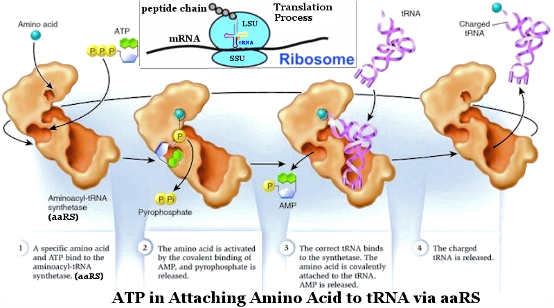
  ATP + H₂O ADP + P_i + 0.32 ev ----- (19).
  However, when ATP supplies are running low, it takes over the function of ATP production by running the process backward.
  
  Figure 17 shows 4 steps of the pump in maintaining the concentration gradient.

  The pump binds 3 intra-cellular Na+ ions as it has a higher affinity for Na+. ATP is hydrolyzed leading to phosphorylation of the pump. The process induces a conformal change and releases of the Na+ ions. The pump binds 2 extracellular K+ ions. This causes the de-phosphorylation of the pump, reverting it to its original state, thus releasing the K+ ions into the cell, and the process repeats itself.

  Figure 17 Sodium Pump in Action [view large image]

  Figure 17 also suggests a possible reverse direction to produce ATP. It involves only the backward direction from (3) to (2), the shape of the pump and concentrations remain unchanged. The process promotes the ADP ground state to the ATP meta-stable state (see insert in lower left corner). In effect, the pump just serves as an enzyme to speed up the backward reaction.

  And so it turns the system into a state of thermodynamic non-equilibrium.



If in the beginning of life, only the simpler sodium pump was available to produce ATP, then it would explain the chemical composition in the Interstitial Fluid (the body fluid outside the cell, i.e., the internal sea in modern life) which has the similar high proportion of Na+, Cl- as in sea water (Figure 19). Modern life retains the original environment where it was born. The saline bag in ICU is a morbid reminder for the role of NaCl in life. In Figure 18, Left : non-living pre-biotic micro-system; Center : intermediate state, relative equal contributions of free energy and entropy; Right : a living organism with basic cellular structures.

Figure 18 Pre-life to Post-life [view large image]

• The energy requirement to run the reverse process in Eq.(19) can be obtained from Sun light, or :
  • Electronic level dissociations in covalent or ionic bond of 4.5 ev from H₂, 4.2 ev from NaCl, ...
  • Vibrational level de-excitation of ~ 1 ev from diatomic molecules.
  • Rotational level de-excitation of ~ 0.2 ev from diatomic molecules.
  • Hydrogen bond of 0.25 ev (for water-water), ...
  • and up to ~ 1.5 ev in some redox potentials.

  		Thus, the starting point of life could be the establishment of suitable Na+/K+ gradient. It could occurred without oxygen (anyway, it was absent 4.3 billion year ago), but it still needs the Sun to provide the energy directly (~ 2 ev from the infrared light) or indirectly through excitation of the molecules.
  Figure 19 Sea Water and Life [view large image]	Figure 20 Origin of Life [view large image]	Of course, this is only a hypothesis. There are various theories such as the LUCA and other recent works. They could be complementary, working together to reveal the Origin of Life.

Figure 21 Transition to Life [view large image]

Figure 22 shows a version of LUCA completed with all the essential parts and the life sustaining process from DNA transcription to protein production. It also indicates the flow of information and energy from/to the environment. This is just the process of entropy dissipation as mention earlier. The original article "Key Steps in the Early Evolution of Life from the Origin of Protein Synthesis to Modern Cellular Life" is a long long discourse on the origin of life starting from the RNA world to LUCA. It contains a lot more detail than the sketch presented here. In this article, it is the chemosynthesis which uses inorganic molecules (such as iron, hydrogen, sulfur, and methane)

Figure 22 LUCA [view large image]

as a source of energy and convert them into organic substances. The simple organism consumed the chemicals from the environment and employed enzymes to speed up chemical reactions, which released energy into phosphate bonds carried by ATP or other similar compounds. This scenario is more suitable for Hydrothermal Mounds origin of life as opposite to "The Hot Spring Hypothesis". (see "Bacterial Metabolism" for various ways).

Go to Top of Page to Select
 or to Main Menu