Fluid Dynamics and the Navier-Stokes Equations

Spiral Flow 2 and Density Wave (2022 Edition)

	While there are many types of spiral as shown in Figure 17d, it is the equations for fluid dynamics (the Navier-Stokes Equations) that dictates a particular one. There is a subtle difference for adopting spherical coordinates in the explicit expression for u and thus selects a different type of spiral (see "Formulas").
Figure 17d Types of Spiral [view large image]	In spherical coordinates the Navier-Stokes Equations can be expressed as :

1. The equation of motion per unit mass of the fluid (see Figure 17e for the explicit notations) -
   


2. Continuity equation per unit mass of the fluid -
   

   Figure 17e Spherical Coordinates and Formulas [view large image]	This angular motion has no source or sink (for the fluid) just swiveling round and round. It is the radial component of Eq.(23c) that generates or drains the fluid as described in an example later.

   
   

   	Conservation of energy equation per unit mass of the fluid -
   Figure 17f Fermat's Spiral [view large image]

The appearance of the spiral is determined by the constants of integration:


• The value of B determines the winding of the spiral. As dr/d = B/r is the relative rate of change between r and , a small value of B/r makes the winding very tight and vice versa (at the limit of circular motion B = 0). This is in contradiction of the appearance of the Milky Way for which the separation between arms is getting larger progressively.
• The solution also admits another spiral arm with -, i.e., winding in opposite direction (see curves on the right of Figure 17f). The sign of B, i.e., B > 0 or B < 0, has the effect on the winding direction - whether it turns to the left or right.
• The spiral can assume a broad sweeping pattern much like the hurricane in Figure 17g instead of one slim locus. Such appearance is encoded by a range of different value of "B" in Eq.(23g).
• The angular momentum for the spiral arm is defined by L₁ = r² (d/dt),
  for the other arm winding in opposite direction L₂ = -r² (d/dt).
  The total momentum L = L₁ + L₂ = 0 indicates that the principle of conservation of angular momentum is upheld. The system neither creates nor destroys angular momentum. Thus, spiral arm in galaxies always appears in pair as shown in Figure 17h.

		For the barred spiral like the Milky Way in Figure 17h, the constant A in Eq.(23i) is determined by the length of the bar; while A = 0 is for the case of true spiral galaxy such as NGC2997. It turns out that the formation of spiral arms in galaxy is more complicated than this simple minded approach, which would produce tightly wound spirals (within 500 million years) in contrary to observation (see more in Theory of Spiral Arm Formation).
Figure 17g Hurricane [view large image]	Figure 17h Barred Spiral	These different cases are shown in the diagrams below [view large image] :

                       

Followings provide demos for some applicable cases in the real world :


1. Spirals toward the black hole at the Milky Way center (NOT the spirals many kpc further out, see Figure 17i) -
   
   • The constant "B" is estimated by reading off the variation of r ~ 3 pc corresponding to turning the spiral by 180⁰, i.e., 3.1416 in radian from Figure 17i,b. Substituting the data to Eq.(23j) yields B ~ 1.4 pc².
   • Figure 17i,b also indicates that the radial velocity u_r ~ 250 km/s at r ~ 0.4 pc. By applying Eq.(23g), the angular velocity
     ru ~ 28 km/s << u_r ; thus the centrifugal force can be neglected in the following calculation.
   
   Now The mass of the black hole at the Milky Way center can be estimated via Eq.(23c) :

   Figure 17i SgrA* Spirals [view large image]

2. This example is about barred spiral galaxy, which is a spiral galaxy with a central bar-shaped structure made of stars (see Figure 17j). Bars are found in up to 70% of spiral galaxies (mostly in the last 7 billion years of the cosmic history). They affect the motions of stars, dust and gas. It is believed that bars act a bit like a funnel, pulling matter into the bulge from the disk.

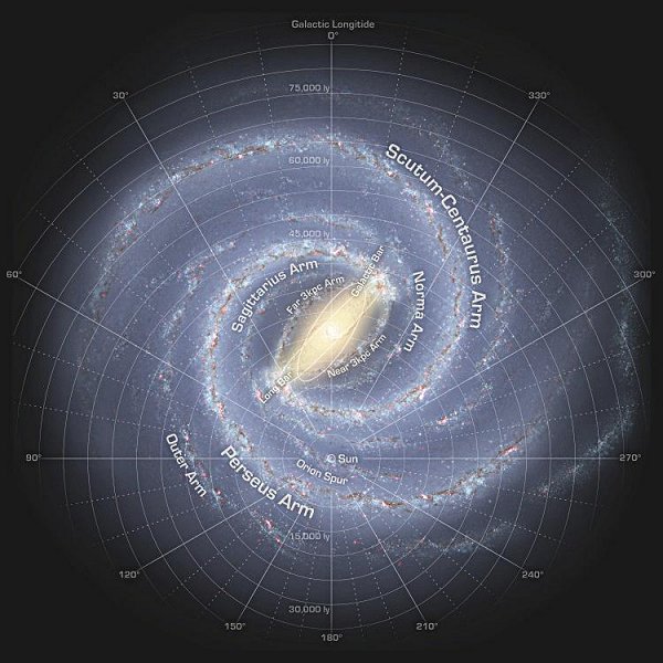
   In barred spirals, there is a bar of stars runs through the central bulge. The arms of barred spirals usually start at the end of the bar. It is suggested that galactic bars develop when stellar orbits in a spiral galaxy become unstable and deviate from a circular path. The tiny elongations in the stars' orbits grow and get locked into place, forming a bar. The bar becomes even more pronounced as it collects more and more stars in elliptical orbits. Eventually, a high fraction of the stars in the galaxy's inner region join the bar. This process is said to be demonstrated repeatedly with computer-based simulations (see "Instability").

   Figure 17j Milky Way Bar [view large image]

   Figure 17j shows the structure of the inner Milky Way including : the bulge, the long bar (origins of the spiral arms at its ends), an additional galactic bar, and the "3-kpc arms" - the near one is inside the Norman arm, both 3-kpc arms are devoid of stars.

   
   Figure 17k,a idealizes Figure 17j into a sketch from which data are collected to compute the velocities from Eqs.(23i) and (23g) :
   
   
   • The 2005 data by NASA measures the size of the bar to be 9 kpc (see visualization of parsec, pc). Thus the distance from its center r₀ = 4.5 kpc. This is the distance to the center at = 0. Thus, according to Eq.(23i) r²/2 = A + B, A ~ 10 kpc².
   • For ₁ = (see Figure 17k,a), r₁ ~ 9 kpc, from which B ~ 9.5 kpc².

   Then from Eq.(23g), ur0 = [B/(r0)2](ru)0 gives ur0 ~ 0.5 (ru)0, where (ru)0 ~ 220 km/sec at a distance of 4.5 kpc according Figure 17k,b (see "SB Galaxies in GR"). These data also show that it takes about 140 million years to complete one rotation. Thus at this point, about 75% of the rotational energy disappears into the sink prescribed by Eq.(23c) implicitly (+ the centrifugal force). Supposedly, such mass-energy is re-used

   Figure 17k Barred Spiral [view large image]

   to power the change of stellar orbits into elongated shape.

3. This example would derive the radial velocity u_r at the center and at its eye's wall of a cyclone (called hurricane in North America). Thus, r ~ 0 for both cases; and according to Eq.(23g), i.e., u = (r/B)u_r , u can be neglected in comparision to u_r (see Figure 17l,a in which the coordinate should be turned upside down for normal viewing). This diagram shows that the mass-energy is drained to the sink as all spirals do, but it eventually returns to the atmosphere at the top of the funnel. This is a major difference from the black hole at the Milky Way center (see example one) into which the mass-energy disappears without a trace.
   
   From Eq.(23c) :

   Figure 17l Profile of Cyclone [view large image]

   See Figure 17l,b for data. This kind of analysis is also applicable to the drain in the sink although on a much smaller scale.



4. The category 5 Katrina Hurricane is used to calculate the radial velocity u_r at the wall of the eye. On August 28, 2005 it was in southeast Louisiana with the following data as shown in Figure 17m,a :
   
   
   • The radius of the eye r_e ~ 25 km.
   • A maximum wind speed ru ~ 290 km/h at the eye's wall r_e.
   • The size of Katrina ~ 600 km.

   	The constant "B" is estimated by reading off the variation of r ~ 23 km corresponding to turning the spiral by 3600, i.e., 2X3.1416 in radian from Figure 17m,b. Substituting the data to Eq.(23j) yields B = r2/2 ~ 42 km2. Then the radial velocity at the eye's wall can be calculated via Eq.(23g) : ur = [B/(re)2](ru)re ~ 20 km/h.
   Figure 17m [view large image] Profile of Hurricane Katrina	Comparing to ~ 10 km/h at the center (see cyclone).

		compressed gas triggers star formation and helps to explain why we see the concentration of bright young stars and clusters in the spiral arms. Figure 17n is a schematic diagram to illustrate the action of a density wave, which causes stars and interstellar gas and dust to bunch up temporarily when the two different types (the high density wave and the spiral of gas and dust) of rotations coincide (in phase), with the spiral arm being the result of a temporary compression of material (Figure 17o).
Figure 17n Density Wave Theory	Figure 17o Density Wave Illustration [view large image]

Some further elaberations (see Figure 17n) :


1. The density wave is represented by a disk of gas/dust rotating with constant velocity (see the white straight line in Figure 17n).
2. When an additional gas/dust spiral (in the form of Fermat's spiral, for example) turning in step (rotating together, i.e., co-rotation) with the density wave disk, there would be a much longer period for materials in the two systems to merge (to compress) producing higher density and higher rate of star formation.
3. Such events usually happen in two places - one spot is near the center at the maximum of the combined rotational veclocty (called "Lindblad resonance" as shown by the yellow curve in Figure 17n); the other one is further out at the co-rotation circle where the two systems move in unison. (see Figures 17n and 17o,a).
4. Lot of short-lived OB stars born and die inside the region of higher density. Since these stars are very luminous, it is actually them, rather than the higher density region, that we observe as the spiral features. However, there is enough older stars to move out of this higher density region to define the over-all shape of the spiral arm (see Figure 17o,b).
                                                     (click me) --- Courtesy of Wikimedia Commons

Figure 17p Spiral Arm [view large image]	which has a maximum at r = 1/k. In comparison to the Kermat's spiral with no F, B = A + r2/2, which has no maximum.

Figure 17q Angular Velocity of Spiral Arm [view large image]	Figure 17q plots u as function of r for k = 0.3, 0.4, 0.5. These curves (except the dubious case for k = 0.3) are similar to the total angular velocity in Figure 17n (the yellow curve) by the density wave theory.

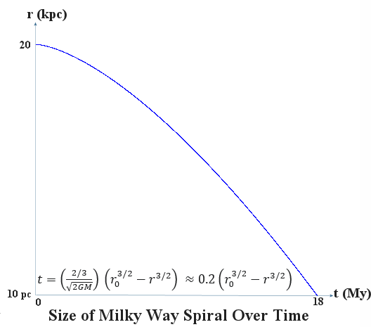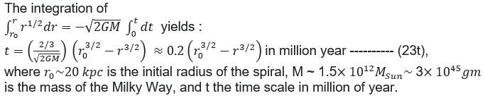	Research into the mechanisms that drive the evolution of spiral arms is still in its infancy, while Figure 17r shows
Figure 17r Spiral Evolution	that the life time of the spiral could be about 18 million years (seems to be too short ???). Anyway, Eq.(23t) indicates that heavier mass M or smaller initial radius r0 has the effect of reducing the life time. For example, if we bump up r0 to 100 kpc, then the life time becomes 200 My.

Now a few coments :


• Figure 17p compares the modifier Kermat's spiral with the Milky Way and NGC 3184, in which different colors represent different frequency of the electromagnetic wave.

Applying Eq.(23o) back to F in Eq.(23n) shows that F e-kr, which has the characteristics of a shear force weakening progressively outward. Actually, this F = -kruur is proportional to the Coriolis force (per unit mass) FC = -2(uur), which is orthogonal to both the r and directions (see Figure 17s). Thus, the extra kr/2 factor is incorporated to account for the differential rotation of the fluid. There are 3 cases of the modifier Kermat's spiral with A = 0, B = 1.4 kpc2 :

Figure 17s Coriolis Force

For k = 0.3, the winding is too tight in comparison to the real cases. For k= 0.4, the shape closely matches with observations. For k = 0.5, the spiral seems to open up too much, but see a more recent example with k = 0.55. Thus, only a small range of k can reproduce a realistic spiral arm (see "Milky Way, Facts").

• It is now apparent that in the density wave theory, the constant (rigid) rotation of a higher density disk somehow imitates the effect of the Coriolis force, while the angular velocity of the gas/dust has its correspondence in the modified Kermat's spiral. The agreement in total angular velocity for both cases is evident in Figure 17n and Figure 17q.

		The Intracluster Medium (ICM) in galaxy clusters is a hot plasma with temperature range from 10 - 100 Mk (million degree Kelvin). Its X-ray emission from the Perseus super-cluster has been measured as shown in Figure 17t. The image shows a cold front with 30 Mk and a radius of ~ 730 kpc. The two shape edges are interpreted as abrupt jumps in density controled by intergalactic magnetic fields. Alternatively, the picture is also consistent with the Theory of Modified Kermat's Spiral (MKS) as shown in Figure 17u with parameters A = 0, B = 1.4, and k = 0.55. The turning point (the kink in lower left of Figure 17t) is at r = 1/k.
Figure 17t Super-Cluster Perseus [view large image]	Figure 17u MKSpiral [view large image]	Since the turning point (the maximum + in spherical coordinates) for this case is ~ 700 kpc. The unit for the length scale in the theory of MKS should be 385 kpc.

See "X-ray astronomy comes of age" for info about the Perseus Super-cluster.

Go to Next Section
 or to Top of Page to Select
 or to Main Menu