| Home Page | Overview | Site Map | Index | Appendix | Illustration | About | Contact | Update | FAQ |
| ---------- (7) |
 .
. | ---------- (8) |
 | ---------- (9a) |
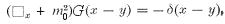
 (x - y) is the delta function.
 , which is visualized as the propagation of virtual particles from x to x' with an infinite range of momentum via the Fourier transform (Figure 01e, and see formula below). The particle at space-time point x has x
 = (it, x), x = (it, -x). Similarly for the source at y.
 |
 |
The 4-momentum k is associated with k = (iE, k), k = (-iE, k). The two particles interact via the virtual particles with different values of k (see Feynman diagram in Figure 01f). For (x - y)2  o the separation is said to be time-like or light-like meaning that the two particles can connect, otherwise they are space-like and cannot communicate with each other. It is forward in time for t > t' ; the reversed is called backward, which is interpreted as forward for anti-particle. Other often used notations are kx = kx = Et - kx, and d4k = dE d3k (all in natural unit with c = o the separation is said to be time-like or light-like meaning that the two particles can connect, otherwise they are space-like and cannot communicate with each other. It is forward in time for t > t' ; the reversed is called backward, which is interpreted as forward for anti-particle. Other often used notations are kx = kx = Et - kx, and d4k = dE d3k (all in natural unit with c =  = 1). = 1).
|
Figure 01e Fourier Transfrom |
Figure 01f Feynman Diagram |
Negecting the distinction on the bare mo and renormalized mass m for the moment, the solution for Eq.(9a) is (see "contour integral" for an important step in the derivation) : |
 |

|
Figure 01g Feynman Propagator [view large image] |
The Feynman propagator has the important feature that includes the anti-particle as going backward in time with negative energy (in the second term), while the first term is for particle going forward in time. |
 k(x) in the Feynman propagator can be replaced by any quantum field (x) in the vacuum expectation value of its product, i.e., iF(x-y) = <0|T(x)(x')|0>, where T is called the time-order operator. It is used to arrange the later time on the left, e.g., t > t' in the above example. This operation is to insure that a particle has to be created before it gets destroyed.(x), (x')] = iF(x-x') for time-like separation, and = 0 for space-like.F(x-x') is divergent as k
  . However for simple tree diagram such as the one in Figure 01f, the conservation of 4-momenta with the real particles (the pi's) presents a factor of
(k - p4 + p2), and (k - p1 + p3) to avoid the divergence in the integration. There would be no such luck in the loop-diagrams.
. However for simple tree diagram such as the one in Figure 01f, the conservation of 4-momenta with the real particles (the pi's) presents a factor of
(k - p4 + p2), and (k - p1 + p3) to avoid the divergence in the integration. There would be no such luck in the loop-diagrams. as derived from the Green's function of the Dirac equation :
 | ---------- (9b) |
 are the gamma matrices associated with the fermion (see "Derivation of the Dirac Equation").
 ; it is equal to 1 for free field, 0 for a point source, and depends on the structure of the source in general. The renormalized field, mass, and energy are
 and EnR = Z-1Eno respectively. The physical mass mR is the experimentally observed mass, mo is an unspecified parameter (called "bare mass") which together with Z-1 determine a value in agreement with experiment. Since Z-1 is infinite for a point source, mo has to be slightly more or slightly less infinite to yield a finite value for mR. This technique of replacing the ignorance in detailed structure of the source by measurement is the more general definition of renormalization, although it is now more often referred to as the method to cancel the infinities in quantum field theory. For example, it involves a many-body Schrodinger equation to compute the viscosity in the Navier-Stokes equations. Since it is impossible to obtain the solution for such a complicated system, its value is determined by experiment instead. A renormalizable theory is one in which the details of a deeper scale are not needed to describe the physics at the present scale, save for a few experimentally measurable parameters (see more in the section about "Renormalizable Theories").