 |
A classical electron moving around a nucleus in a circular orbit has an orbital angular momentum, L=mevr, and a magnetic dipole moment,  = -evr/2, where e, me, v, and r are the electron´s charge, mass, velocity, and radius, respectively. A classical electron of homogeneous mass and charge density rotating about a symmetry axis has an angular momentum, L=(3/5)meR2 = -evr/2, where e, me, v, and r are the electron´s charge, mass, velocity, and radius, respectively. A classical electron of homogeneous mass and charge density rotating about a symmetry axis has an angular momentum, L=(3/5)meR2 , and a magnetic dipole moment, = -(3/10)eR2, where R and are the electron´s classical radius and rotating frequency, respectively. The classical gyromagnetic ratio of an orbiting or a spinning electron is defined as the ratio , and a magnetic dipole moment, = -(3/10)eR2, where R and are the electron´s classical radius and rotating frequency, respectively. The classical gyromagnetic ratio of an orbiting or a spinning electron is defined as the ratio
|
 cl =
cl =  /2.
/2.


 /2
/2 ), where
 a
a


 =
=  /dt),
/dt), S = 2
S = 2
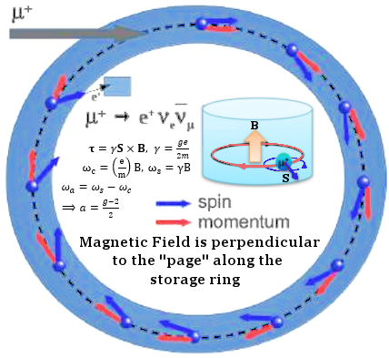
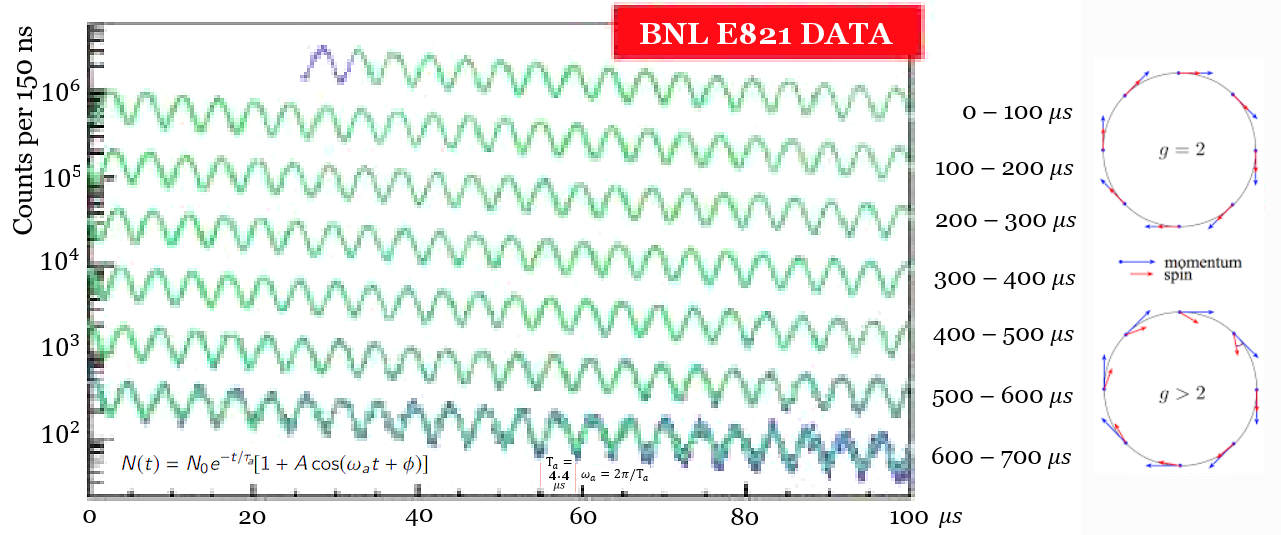
 s. However, the detectors lining along the inside of the storage ring will experience cycle of maximum and minimum as the positrons point toward and then away from them with frequency
  )].
)]. 


 g) between isotopes, many common QED contributions cancel out owing to the identical electron configuration, making it possible to resolve the intricate effects stemming from the nuclear differences.
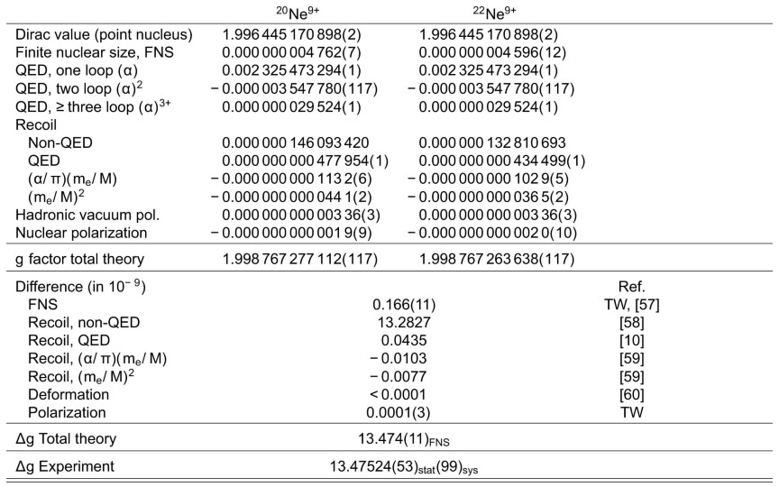

 L so that the moments pointing at different directions.
 ] + 0.5 ---------- (1)
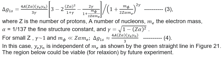
 by the following formula for the bound electron in 1s state (see more details in "Fifth-force search with the bound-electron g factor") :

