Relativity, Cosmology, and Time

Standard Cosmology

• The space-time interval is associated with the Robertson-Walker metric. It has three forms depending on the curvature of the 3 dimensional space:
  
  ds² = c²dt² - R(t)² (dr² + w² (d² + sin² d²)) ---------- (17)
  
  where w = sin(k^1/2 r) / k^1/2, k (in unit of cm^-2) can be considered as the total energy of the universe, and R(t) is called the scale factor. It expands the coordinate grid as a whole with the expansion of the universe. Such grid is referred to as comoving coordinates. Thus if we denote dr to be the comoving distance between two points, then dx = R(t)dr would be the physical distance actually measured by a ruler at time t.
  
  For flat space with zero curvature, k = 0, and w = r, where r ranges from 0 to infinity.
  For closed space with positive curvature, k > 0, w = sin(r), where r ranges from 0 to 2.
  For open space with negative curvature, k < 0, w = sinh(r), where r ranges from 0 to infinity.



• In term of the Robertson-Walker metric and with the energy-momentum tensor T₀₀ = , the gravitational field equation can be written in a form (called Friedmann Equation) similar to the energy equation (K.E.+P.E.=E):
  
  (dR/dt)² - 8GR² / 3 = - kc² ---------- (18a)
  
  which can be re-arranged into the form:
  
  H² - H₀² = -k² c²/R² ---------- (18b)
  
  where H(t) = (dR/dt) / R is the Hubble's parameter, = / _c is the density parameter, and _c = (3 H₀²) / (8G) ~ 0.9x10^-29 gm/cm³ is the critical density, which corresponds to the total energy density for a flat universe.
  
  for flat space, = _c, = 1, k = 0;
  for closed space, > _c, > 1, k > 0;
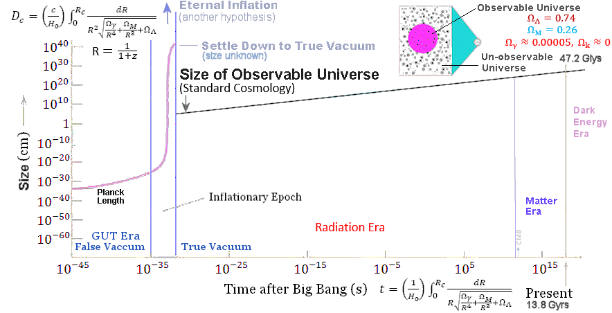
  for open space, < _c, < 1, k < 0.

While the Hubble's parameter H(t) depends on time t, it is denoted as H₀ at the current epoch t₀, and called the Hubble's constant; T = 1/H₀ is called Hubble's time - the time since the Big Bang. The scale factor for the current epoch is often taken to be unity for convenience, i.e., R₀ = 1 by equating the radius of the universe r₀ = (9GM/2)^1/3 t₀^2/3 according to Eq.(19a). The formalism assumes the ratio M/(r₀)³ to be a constant for a homogeneous and isotropic universe. Thus, the scale factor R is the same for both the unobservable and observable expansion but corresponding to different radius r₀ (see Figure 10a1, and text below). We can also express R = (t/t₀)^2/3 to get rid of M/(r₀)³ altogether.

		In the theory of inflation (Figure 10a1), the radius of the universe had been stretched to an enormous amount in a very short time. The scale factor R is derived by the theory of standard cosmology starting from the end of this brief period. The size of the observable universe is restricted by the event horizon : DH = c x t (Figure 10a2, also see "History of the University").
Figure 10a1 Cosmic Inflation [view large image]	Figure 10a2 Event Horizon



• More generally, when several types of matter-energy coexist in the universe, the following consistency relation (for k = 0) must be satisfied:
  = _jj = 1
  where the sum is over the various types of matter-energy. Present cosmological observations yield:
  
  _b ~ 0.04 for brayons (ordinary visible and nonluminous matter),
  _d ~ 0.26 for exotic dark matter,
  ~ 0.7 for dark energy,
  ~ 5 x 10^-5 for photons (radiation).


• For a homogeneous and isotropic (matter only) universe = M / (4R³r₀³/3) ---------- (18c)
  
  where M may be interpreted as the mass within the radius r₀ with the ratio M/(r₀)³ to be a constant, then Eq.(18a) becomes:
  
  (dR/dt)² - 2GM / Rr₀³ = -kc² ---------- (18d)
  
  The solution for this equation is:
  
  for k = 0,     R = (9GM/2r₀³)^1/3 t^2/3,      t = 2/3H ---------- (19a)
  
  for k > 0,     R = R_o (1 - cos(k^½µ)),     ct = R_o (µ - k^-½sin(k^½µ)) ---------- (19b)
  where R_o = GM / |k|c²r³, and µ is defined by c dt = R(µ) dµ.
  
  for k < 0,     R = R_o (cosh(|k|^½µ) - 1),     ct = R_o (|k|^-½sinh(|k|^½µ) - µ) ---------- (19c)

For the radiation (relativistic matter, i.e., particles with kinetic energy higher than the rest mass energy) dominated universe, the radiation pressure p = /3. Starting from the thermodynamic relation dU = -pdV, where U = V, and V is the volume of the system (the universe in this case), it can be shown that 1/R⁴, Eq.(18a) (for the case k = 0) becomes dR/dt 1/R, the solution for which is R t^½. Incidentally, since the temperature T is related to the energy density as T⁴, thus T 1/R. See simply mathematical derivation below :

dU = dV + Vd = -pdV (p + )dV = (4/3)dV = -Vd (integrating) n(V/V₀) = n[(R/R₀)³] = -(3/4)n (/₀) = ₀ [1/(R/R₀)⁴]
-- QED.


• Observationally, the red shift z caused by the cosmic expansion can be expression in terms of the scale factor R [see Figure 10b1, which shows the red shift of the Balmer series of the hydrogen line spectra (dark lines, denoted by H, ...) superimposed on the continuous spectra (colored), the arrows indicate the direction of increasing values for the corresponding variables]:
  
  z = ₁ / ₂ - 1 = R(t₂) / R(t₁) - 1     or     z + 1 = ₁ / ₂ = 1/R(t) ---------- (19d)
  
  

  where t2 denotes the current epoch, 2 is the red shifted wavelength (as measured on Earth), 1 is the wavelength of the original spectral line that was emitted at time t1 in the distant past, R(t2) is often taken to be R0 = 1 for convenience, then R(t1) is less than 1 in the past and is often just denoted as R(t). The quantity (z + 1) can be considered as the amount of stretching during the intervening time for the light to travel from there to here. The relativistic expression for z+1 (In terms of the recession velocity v) is: z + 1 = [(1+ v/c) / (1- v/c)]1/2. The red shift z becomes infinity at the event horizon when v = c, and z ~ v/c for v << c.

  Figure 10b1 Cosmic Red Shift [view large image]

  
  
• The cosmological model in the last section is the oldest and over-simplified before the discovery of dark matter and dark energy. Since then a number of revised models have been investigated and can be summarized in a "Cosmic Triangle" (Figure 10b2). Its three sides are identified with the scale of the density parameters : _mass (for all matter - dark and brayonic), _{dark energy}, and _curv (associated with the curvature of space). The location of the various models are depicted in Figure 10b2 and explained briefly below in order of antiquity.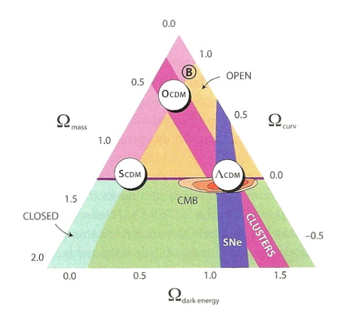

1. Model B - This model includes only the baryonic matter. The universe seems to be open before 1970s, and nobody knew the cosmic expansion is accelerating. 2. OCDM - This is the model when cold dark matter was favored by observation in the 1970s. The "O" represents "Open" universe, which was still embraced by many astronomers. The cosmic age is constrained by the age of star cluster. 3. SCDM - It stands for "Standard Cold Dark Matter" with no dark energy but now they got a hint that the universe is flat. 4. CDM - This is the most current model constructed after the discovery of dark energy in the 1990s by observing the Type Ia supernova explosion. It fits all the astronomical observations including the CMBR.

Figure 10b2 Cosmological Models [view large image]



• There are various kinds of cosmic distance according to the way it is measured (see Distance Measures in Cosmology by David Hogg).

  		They have different dependence on the redshift z, and yield different limiting values as z . Table 03 below is a summary of all these distances. The formulas in terms of z are derived from the "matter only" flat-space model, which can be expressed in close (analytic) form. The more realistic solution including dark energy has to be evaluated numerically as shown in Figures 10c. Figure 10d depicts the lookback dis-tance and time etc pictorially (not to scale). The Hubble distance in Table 03 is defined as DH = cT = 13.7x109ly
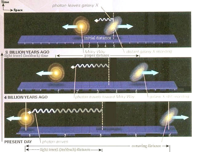
  Figure 10c Types of Cosmic Distance [view large image]	Figure 10d Lookback Distance and Lookback Time [view large image]

  
  The comoving distance is the fundamental distance measure in cosmology since many others can be derived in terms of it. Within the framework of general relativity, it can be expressed as:
  
  D_C = D_H dz' / [_M(1+z')³ + _k(1+z')² + ]^1/2
  where _M = 8G₀/3 H₀², _k = -kc²/ H₀², and = c²/3 H₀².
  
  Thus, a theoretical comoving distance can be computed as a function of the redshift z from the density parameters 's resulting in many cosmological models with different combinations of these parameters. Similarly, the lookback or light travel distance is given by:
  
  D_T = D_H dz' / (1+z')[_M(1+z')³ + _k(1+z')² + ]^1/2
  
  The difference between D_C and D_T is that the former is derived from the conformal time , while the latter is related to the regular time t. The conformal time is introduced because of a peculiar feature in cosmic expansion. It has been mentioned that the physical distance dx is related to the comoving distance dr by the formula dx = R(t)dr. It follows that the velocity dr/dt = (1/R)dx/dt, then for dx/dt = c, dr/dt > c when R < 1. The conformal time defined by dt = Rd is invented to address this problem of exceeding the velocity of light. Since by using the conformal time dr/d = dx/dt, it would not have the problem when dx/dt = c. In the comoving frame, the mutual recession of two objects is viewed as the expansion of the coordinate grids (see Figure 10d).
  
  Table 03 lists the various types of cosmic distances with formula of their dependence on the scale factor R (or red shift z).
  
  

  Type of Distance	Definition	Function of R = 1/(1+z)	Size / Age of the Universe
  Comoving / Conformal (DC)	From here to there at the current epoch		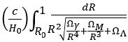47.2x109 lys (Rp=1)
  Coordinate / Proper (DP)	From here to there in the past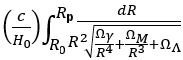
  Angular Distance (DA)	Intrinsic linear size / angular size		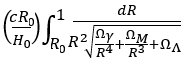0
  Light Travel / Lookback (DT)	Light travel Distance from source Re to here		13.7x109 lys (Re=0)
  Light Travel / Lookback Time (T)	Light travel time from source Re to here		13.7x109 years (Re=0)

  Table 03 Types of Cosmic Distance

  The diagram (Figure 10e) below lists some cosmic parameters as a function of the red shift z. It includes :
  
  H - Hubble constant in km/sec-Mpc,
  r-comov - distance (to us) according to Hubble's law in Mpc,
  dm - density of matter in % of the total cosmic mass-energy,
  age - age of the astronomical object in Gyr,
  time - traveling time to reach us in Gyr,
  size - angular size scaling in kpc/1^",
  angle - angular size of 1 kpc astronomical object in arcseconds;
  1 Gly = 1,000,000,000 light years = 9.461x10²⁶ cm,
  1 Mpc = 1,000,000 pc = 3,261,566 light years = 3.08568x10²⁴ cm,
  1 Gyr = 1,000,000,000 years.
  
  

  Figure 10e Relation of Cosmic Parameters to the Red Shift z [view large image]

  The above data were computed with H_o = 67.15 km/sec-Mpc, _m = 0.317, = 0.683 according to the latest observation from ESA/Planck. The program to calculate cosmic models with various input data is available online known as "Cosmic Calculator".
  
  

  	The diagram on the left of Figure 10f shows the Type Ia supernova raw data up to a redshift of about 1.5 (or down to 0.4 in term of the scale factor). After various adjustments for these observations, the data points agree remarkably with a theoretical curve as shown in the diagram on the right. This model is computed with matter-energy composition and spatial curvature estimated by WMAP.
  Figure 10f Type Ia SN Data [view large image]	Note that (by flipping the curve to the left) Figure 10f represents a short segment of one of the cosmic models in Figure 10g.

  The various data reductions include:
  
  1. Change redshift to scale factor.
  2. Correction for over estimate of luminosity distance by expansion-induced dimming of light.
  3. Conversion from coordinate distance to light travel time or lookback time.
  4. Average over multiple galaxies.
  
  

  Figure 10g shows the three types of universe - open, flat, and closed. Universes that are too far above the critical divide expand too fast for matter to condense into stars and galaxies; such universes therefore remain devoid of life. Those that fall too far below the critical divide collapse before stars have a chance to form. The shaded area indicates the range of cosmological expansions and epochs in which observers could evolve. By measuring the sum of the angles in a huge narrow triangle with one vertex on Earth and the other two at the points of emission of CMBR (see insert in Figure 10g), the WMAP data yields a value of 180o indicating that the universe is

  Figure 10g Types of Universe [view large image]

  flat. Such conclusion is further supported by the acceleration of Type Ia supernovae, which imply a precise amount of dark energy needed to make the universe flat (with the total matter-energy density equals to the critical density).

  Note: For closed space the sum of the angles in a triangle would be greater than 180^o; it is smaller than 180^o for open space; it equals to 180^o exactly for flat space.

Go to Next Section
 or to Top of Page to Select
 or to Main Menu