Double-slit Experiment, Gateway to Quantum Theory (2020 Edition)

		source of distribution of wave; in other words, if we know the value of the wave function on a given wave front, then we can express its value elsewhere as the sum of contributions from different elements of the wave front in the form of propagating spherical wave, e(2i r/)/r, where r is the distance from the point in question to the element of surface on the wave front, and is the wavelength. Assuming that the slit is very narrow, the two waves from slit 1 and 2 can be represented as: 1 = Ae(2i r1/)/r1 ---------- Eq.(01a) 2 = Ae(2i r2/)/r2 ---------- Eq.(01b) where A is the normalization constant, r1, and r2 are the distance from the slits to the screen as shown in Figure 01, which lays out the x-y plane only, while the z direction is perpendicular to the computer screen.
Figure 01 Double-slit Exp. [view large image]	Figure 02 Wave Magnitude

	1*1 2*2 (A2/r2) ---------- Eq.(02a) 1*2 + 2*1 (2A2/r2) cos[2(dsin/)] ---------- Eq.(02b) The combined magnitude is : P12() = 1*1 + 2*2 + 1*2 + 2*1 (4A2/r2) cos2[(dsin/)] ---------- Eq.(03) The normalization constant A can be evaluated by integrating Eq.(03) numerically over the angle from -/2 to +/2 :
Figure 03 Slit Experiments [view large image]	1 = (8A2/D2)cos2 cos2[(dsin/)] d ---------- Eq.(04)

For the values of d and quoted below, the integral is equal to about 0.390, which gives A = 0.566D. For rapid oscillation of the interference term, i.e., when d >> , the integral approaches a value of /8, giving A2 = D2/ or A = D/1/2 = 0.564D. Then it shows clearly that P12() can be interpreted as the magnitude per unit radian. The experiment was first performed with light by Thomas Young in 1801; thus it is sometimes referred to as Young's experiment. It is rather obvious from Eq.(03) that maxima occur at : d sin = n , where n = 0, 1, 2, 3, ... ---------- Eq.(06a) while the minima are at : d sin = (n/2) , where n = 1, 2, 3, ... ---------- Eq.(06b) By early 20th century technology had been advanced enough to provide low intensity light and its detection. Observation then revealed that the interference pattern is produced in random specks

Figure 04 Double-Slit Experiment [view large image]

(in the detecting film). The pattern emerges only after long exposure (see Figure 04 for a modern version of the sequence of increasing number of photons). The discovery is now understood in the framework of quantum theory as explained below :

• The most obvious aspect of the double-slit experiment is the wave-particle duality. As shown in Figure 03, the detection of wave or particle pattern depends on the experimental setup. Figure 04 shows that the appearance of either particle or wave depends on the number of particles.



The cross terms in Eq.(02b) can be identified to "entanglement" (see Figure 05,b) even though the setup can be reduced to involve only one particle. Therefore, it seems that a single particle can be splited into two in the double-slit experiment. This is one of the weird concept that bothers lot of people. Some text books refer to the interference terms as superposition (Figure 05,a), which is actually the addition of two or more states as will be explained later. Anyway, a measurement will collapse the entanglement (to a point in the double-slit experiment) as well as the superposition (e.g., to a definite state of either spin up or down). What happens in between is unknowable. This is another weird aspect leading to so many "interpretations".

Figure 05 Superposition & Entanglement

BTW, superposition is an "OR" operation involving addition, while entanglement is "AND" operation via multiplication (see "Probability and Information").

• The wave-particle duality persists from electron to molecule comprised as large as 810 atoms (~ 10^-5 cm). The de Broglie relation :
  p = h/ ---------- Eq.(07).
  provides a link between the particle momentum p and wavelength of the matter wave. This equation implies a reciporal relationship between the energy(E) and length(L) scales, i.e., E ~ hc/L or E(Gev) ~ 10^-13/L(cm).



The uncertainty relation (Figure 06) can be derived from Eq.(03) by considering the variation of P12 in one cycle from (dsin/) = 0 to , which yields : d(sin)/ = 1 or d(psin) = h ---------- Eq.(08a) by applying the de Broglie relation in Eq.(07). The uncertainty in the position along x is the distance between the slits, i.e., x = d. The movement of the particle is along the r direction as shown in Figure 01, therefore, the uncertainty of momentum along the x direction is px = p(sin) from which Eq.(08a) turns into the uncertainty relation : xpx = h ---------- Eq.(08b).

Figure 06 Uncertainty Principle [view large image]

It can be shown that the uncertainty relation is equivalent to the commutative relation [x(px) - (px)x] i ---------- Eq.(08c), where the "i" is inserted for realizing an oscillating wave and h is replaced by = h/2.

Similar relations exist for other type of conjugate variables such energy (E) and time (t), i.e.,
Et = h ---------- Eq.(08d).
This formula implies the occurrence of very high energy "virtual particle" for very short time. The phenomenon causes a huge problem for the evaluation of scattering cross section in some processes (see "QED Divergences").

The usual analogy is to an embezzling bank teller who takes money from the till but always replaces it before the auditor comes around. Naturally, the more money is entrusted to the teller, the more frequently the auditor would checks up on her/him. Thus, the opportunity for "borrowed investment" is a constant (money = energy in this analogy to Eq.(08d)).


• The matter wave is governed by the Schrodinger equation, which is derived by quantizing the energy equation E = p²/2m + V, where the linear momentum p = mv and V represents the potential energy. As such, it it suitable only for low energy (non-relativistic) physics because it is not Lorentz invarant. Quantization is the process to find an operator that can satisfy the commutative relation in Eq.(08c). The conjugate variables can be expressed in matrix, while in differential form

  	It shows that starting from a non-linear equation for r, i.e., E = (m/2)d2r/dt2 + V(r), quantization has it linearized into the Schrodinger equation for the wave function which
  Figure 07 1st Quantization [view large image]	admits superposition of its solutions (as another form of solution). Thus, it is the theoretical design and experimental evidences that bring about the weird world of superpostion.

  Figure 07 shows pictorially the classical and quantum views of the hydrogen atom. The nucleus serves mainly as source of the electro-static field e/r² (or V = -e²/r) while it is the electron which turns into standing wave of probability P = ^* (with the up and down of the probability wave represented by colors, see Figure 07).
  
  

  	is also a solution (Figure 08a).
  Figure 08a Superposition [view large image]	Measurement of the wave packet would collapse the superposition into just one of the solutions with probability c*(k)c(k).

  Figure 08b Standing Waves	Figure 08c Coherence	See "Harmonic Oscillator" and "Infinite Square Well".

  The particle usually occupies a stationary state (i.e., the eigen state) at ground level. Superposition is created by interaction with some kind of force. The wave functions in the superposition move in unison (coherence). It only breaks up (decoherence) in the process of measurement. The detector would pick out one of the states according to the probability. This is called the collapse of the wave function in the jargon of "Copenhagen Interpretation". Such concept seems to be alien for some people, and in particular to the pure theorists and philosophers, who are very un-comfortable with such arbitrary rule, i.e., getting the result of a measurement or perception by chance.


• In the discussion above, only the electron in atom and the nucleon in atomic nucleus are quantized. The interacting potential V or field is still in its classical form. The subject of quantization of wave is presented in "Quantum Field Theory". It also has the property of superposition and its collapse in the process of measurement.



• Figure 09 demonstrates the concepts of superposition and entanglement in diagrams and mathematical formula by 2 photons. Photon 1 can exist in 2 polarization states |1₁, and |0₁; while the states of photon 2 |1₂, |0₂ are determined by the order it runs through gate A or B. The superposition can be expressed as :
  

  	|fk = a|1k + b|0k ---------- Eq.(09a), where k = 1, 2 for photon 1 and 2, a and b are the probability amplitude satisfying the normalization condition |a|2 + |b|2 = 1. Entanglement mixes the states of the two photons in the form similar to Eq.(02b) : |m1|n2 = |mn ---------- Eq.(09b)
  Figure 09 [view large image] Superposition/Entanglement	and its linear combination, where m, and n represent the state of the 1st and 2nd photon respectively. In particular, the maximally entangled Bell states are listed in Figure 09,d in which S and T stand for singlet and triplet states. Entanglement is obtained by "Down Conversion".

  Measurement decoheres the superposition/entanglement producing the basis states with certain probability (see for example, the measurement of the singlet in Figure 09,d) :
  P₁₂ = (10|10 + 01|01)/2 ----------- Eq.(10).
  Figure 09,d shows the result of the measurement that would appear 50% of time, the other half would involve the dissolution of
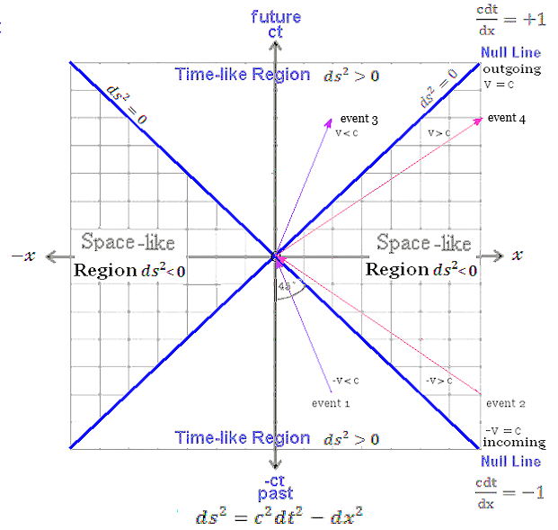
  |01 to its basis states of |0₁ and |1₂. Both the measured results would show up simultaneously no matter how far apart are the members of this pair, measuring one will flip the opposite at precisely the same moment. This non-local influence (objects can influence each other only locally, i.e., distance d ct, according to classical physics) occurs instantaneously, as if some form of communication, which Einstein called a "spooky action at a distance", operates not just faster than the speed of light, but infinitely fast. This phenomena of non-locality has been validated by the "Bell's Theorem" tests. Furthermore, the experiment reveals that it is not possible to predict whether photon 2 goes from A to B or from B to A (because both occur only 50% of the time).
  
  

  Similar experiment was carried out in 2017 with state |12 and |02 represents the "cause-effect" and "common cause" relationship respectively (Figure 10). It shows that these relationships can be mixed in the quantum environment contrary to classical concept. Future experiment is trying to reverse the order of "cause-effect" so that effect comes before cause. It is said that this is one way to move forward to "new physics", to solve the "quantum-gravity" impassse, and to advance the development of quantum computing.

  Figure 10 Causality [view large image]

  BTW, the "cause-effect" relationship is similar to an "OR" operation, i.e., A or B (A precedes B in Figure 10,a). While the "common-cause" is related to the "AND" operation, both A and B occur in parallel. It requires a priori "cause" such as the rain in Figure 10,b to establish the correlation (none otherwise).

  See "In The Quantum Realm, Cause Doesn’t Necessarily Come Before Effect".
  
  

  Figure 10 also reveals that the correlation between 2 events in "cause-effect" relationship requires certain amount of time to establish (as shown in diagram a). Therefore, their separation is limited by the velocity of light which propagates the signal (see Figure 11, the Minkowski space-time diagram shows that events are related only in the time-like region). On the other hand, the 2 events in "common-cause" are linked already, i.e., no need to send signal to relate. In the context of superposition/entanglement, superposition is similar to the "cause-effect" relationship, while entanglement is related to the 2 parallel events in the "common-cause" relationship. It implies that invoking one event automatically connects the other with no time delay (see Figure 10,b). Einstein decried such happening as "spooky action at a distance" which distressed him so much as it violates his cherished idea of "no signal that can move faster than the velocity of light".

  Figure 11 Minkowski Space-time

  Similar to the un-observability of superposition, entanglement is also un-observable. Any attempt to measure these entities would break it up to its basic components, i.e., it never shows up as a whole. There is no hidden variables as verified by numerous tests on "Bell's Theorem".