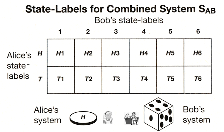
 's and |b's. In particular, SA could be represented by a coin with basis vectors |H (for head) and |T (for tail), while SB is a dice with basis vectors labeled by 1, 2, 3, 4, 5, 6. The combined system (called SAB) has basis vectors shown as the table entries in Figure 01, e.g., |H1, ... |T6. This is the tensor product from merging two vector spaces. Any operator in SA can only act on the first label, same is for SB on the second label. Superposition state in SAB is written as :
Figure 01 Combined System
[view large image]

where |aibj
is the basis vector in SAB with associated probability c*ij cij .


 0.
0.


 i> by an instrument. Since the quantum state |
 > can be a combined system such as the entanglement of many qubits, the entanglement also undergoes decoherence. It is sometimes referred to as transfer of entanglement to the environment.
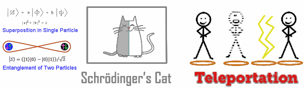
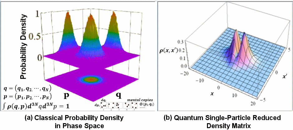


 (x,x'), and why we don't care the other particles, is that all the particles are identical. Therefore, all we need to do is to work out the value for one particle and to multiply the result by N times so that the sum of
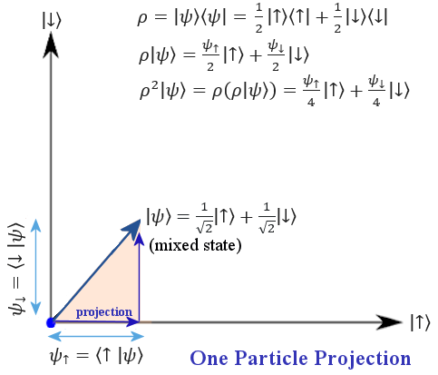
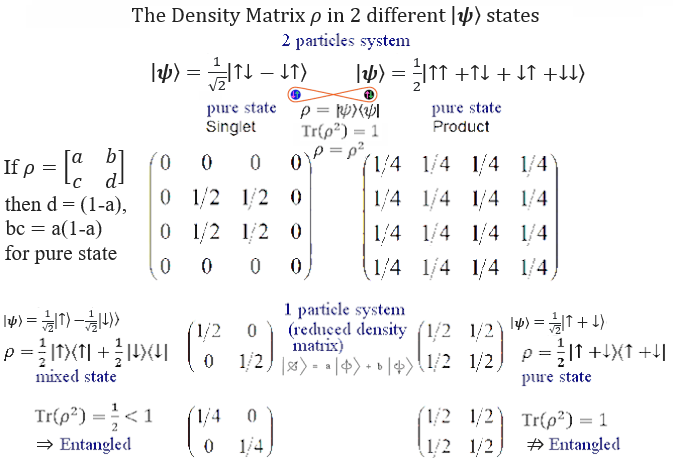

 , and tr(


 i pilog2(pi), where pi represents the discrete probability distribution of some samples.
  )
) n(2) =
  )
)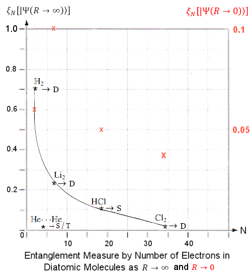
 and ultimately
  N as function of the inter-atomic distance R. The
  0 and
0 and  (at different scale in ratio of 0.1/1).


 (see Figure 03p).


 r = 0, and
  by the de Broglie relation p = h/
 = h/2
= h/2 ; the uncertainty is thus expressed as
 -i
-i
 .
.


 3 -
3 -  0.
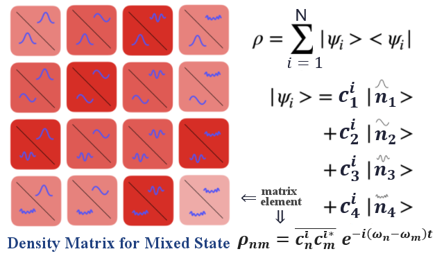
Such system is shown pictorially in Figure 03s4,
the mathematics is summerized below (see "Density Matrix" for the original derivation) :
0.
Such system is shown pictorially in Figure 03s4,
the mathematics is summerized below (see "Density Matrix" for the original derivation) :


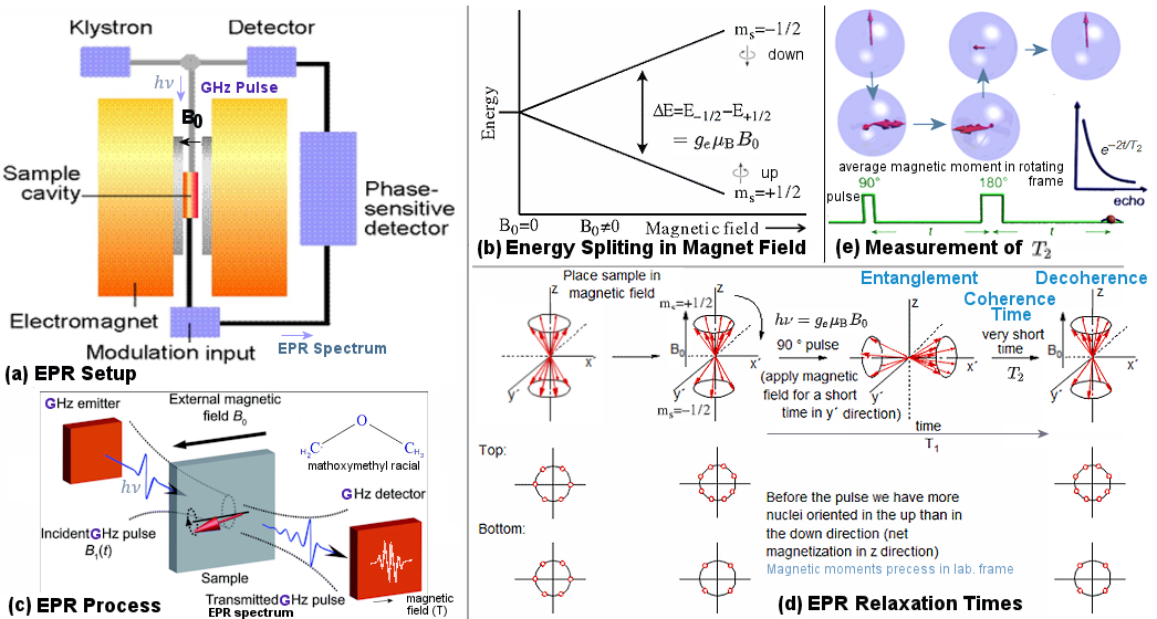
 c, which is the duration from beginning to end of entanglement. This is an important factor in quantum computing where

 BB0, with corresponding energy gap
  =
= 


 , |01
, |01 3, -i
3, -i


 2 + sin2
 |/3)1/2c,


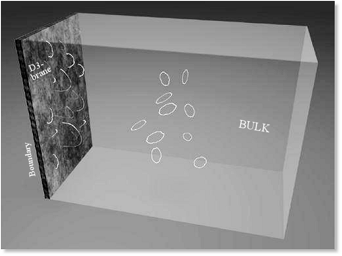
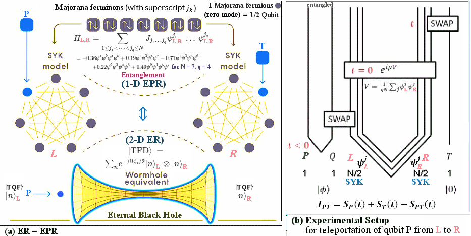
 |m>R is labeled by |n, m>. The eternal black hole is described by the entangled state :
 entropy)" as shown by


 2} c2dt2 +


![[view large image]](I15-81-Hilbert.png)