| Home Page | Overview | Site Map | Index | Appendix | Illustration | Preface | Contact | Update | FAQ |
-only)![]() |
for a homogeneous and isotropic universe when the size of the universe was at the Planck scale of 1.6x10⁻³³cm; then the whole universe can be considered as a small particle (with certain mass and size). By quantizing the dimensionless scale factor R and its time derivative dR/dt, this particle is endowed with a wave property; the corresponding wave function 
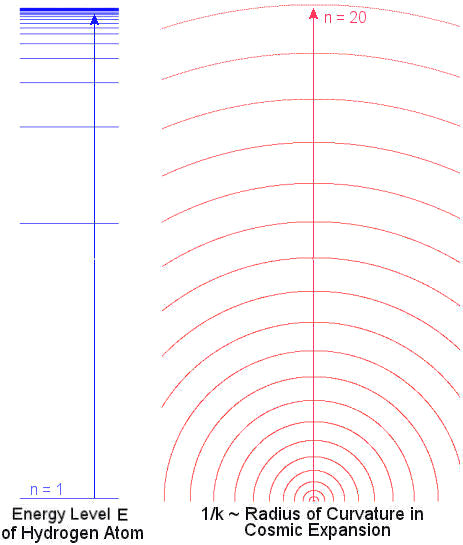
can be interpreted as the probability amplitude at certain value of the scale factor R. It turns out that the resulting wave equation is similar to that for the electron in the hydrogen atom (with different interpretations of the parameters). In particular, the energy in the case of hydrogen atom is now replaced by the spatial curvature k. The transition from its extremely large value to small number corresponding to a nearly flat space can be interpreted as quantum jump to near continuum during the period of inflation. Figure 01a compares the energy levels of the hydrogen atom and the inverse of the spatial curvature (~ radius of curvature) in cosmic expansion. The appearance seems to be in reverse since the correspondence is between E (energy level) and k (spatial curvature), and the plot is for 1/k to make it looking like the expansion of the universe. This formulation is similar to the Wheeler-DeWitt equation, which is also derived from the Friedmann equation with an un-specified potential. |
Figure 01a Energy Level and Cosmic Expansion |
This treatment adopts a potential corresponding to a matter-only universe. The other alternative with "cosmological constant -
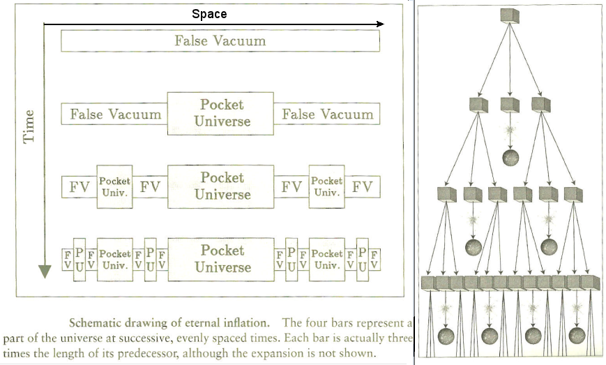
only" is explored in the section on "Quantization of the Empty Universe". |
, where px = m dx/dt is the momentum along the x axis. This equation is satisfied if px = -i
d/dx and operates on a (wave) function
. In order to follow this quantization rule for the case of cosmic expansion, we can assign R to take the place of x and construct an entity having the dimension of ergs-sec = gm-cm2/sec (the dimension of
) such as Mr2dR/dt. Thus the commutative rule becomes:
, which can be satisfied for Mr2dR/dt = -i
d/dR or dR/dt = (-i
/Mr2) d/dR.
/dR2 + (M2r4c2/
2)[(2GM/c2r3R) - k]
= 0 ----- (2)
= R
, this equation can be re-cast to :
/dR2 + (2/R)d
/dR + (M2r4c2/
2)[(2GM/c2r3R) - k]
= 0 ----- (3)
/dr2 + (2/r)d
/dr + (2m/
2)[(e2/r) + E]
= 0 ----- (4)
2)(1/n2) ----- (5)
= [2/(nr0)½] (1/n2r0) e-r/nr0 Ln-1(1)(2r/nr0) ----- (6),
(-1)j[n!/(n-j-1)!(j+1)!j!]xj
2/me2 .![]() |
By substituting k to -E, R to r, M2r4c2/ 2 to 2m/ 2, and 2GM/c2r3 to e2, the quantized Friedmann equation yields :k = (2GM/c2r3)2 (M2r4c2/4 2)(1/n2) = G2M4/r2c2 2n2 ----- (7), = 2[(R/nR0)/(nR0)½](1/n) e-R/nR0 Ln-1(1)(2R/nR0) ----- (8),where R0 = (c2r3/2GM) (2 2/M2r4c2) = 2/GM3r . The Laguerre polynomial and wave function for a few low laying states are listed in Table 01 below (also see Figure 01b).
|
Figure 01b Wave Function |
| n | Ln-1(1)(x) | n(R) |
|---|---|---|
| 1 | 1 | [2(R/R0)/(R0)½] e-R/R0 |
| 2 | 2(1 - x/2) | [2(R/2R0)/(2R0)½] (1 - R/2R0) e-R/2R0 |
| 3 | 3(1 - x + x2/6) | [2(R/3R0)/(3R0)½] [(1 - 2(R/3R0) + (2/3)(R/3R0)2] e-R/3R0 |
| n-1 | n[1 - (n-1)(x/2) + ... (-1)n-1(xn-1/n!)] |
[2(R/nR0)/(nR0)½][(1 - 2(R/nR0) + ... (-1)n-1 (2n-1/n!)(R/nR0)n-1] e-R/nR0 |
/c3)½ = 1.6x10⁻³³cm. However for the Planck mass Mp = (
c/G)½ = 2.17x10⁻⁵gm, its corresponding Schwarzschild Radius rs is equal to twice the Planck length, i.e., rs = 2GMp/c2 = 2Lp implying the initial radius r is inside the event horizon, i.e., the particle is a black hole. It has been shown that such black hole would evaporate rapidly in 10-40 sec (see Black Hole Evaporation) about the scale of the Planck time (see "World of Planck Scale").
| An article in "New Scientist, January 2-8 2016" with the title "Quantum Bounce" postulates that the collapse to black hole can be reversed to ejection from white hole by the space-time loop in the "Theory of Loop Quantum Gravity" (Figure 01c). Calculations show that bigger black hole would take longer to bounce. Thus, the authors are looking for evidences from small black holes more common in earlier history of universe; and that's why we don't see such event nearby. However, nobody would perceive the very slow process that turns the whole universe from its previous collapsing cycle back to the expansion phase today. Such idea is similar to the black hole evaporation (particularly at its very last stage as considering here). Therefore from such perspectives, the event horizon is not a barrier for expansion. |
Figure 01c 3-D White Hole |
See earlier work on "LQG Cosmology". |
|
Anyway, expressing in term of the Planck length, k and R0 can be written in a very simple form : k = 1/(n2Lp2) = 40x1064/n2 cm-2, and R0 = 1 ----- (9). In analogy to the Bohr radius for hydrogen atom, R0r = Lp for n = 1 can be identified as the classical radius of the particle at ground state (Figure 01d), and R0/ 
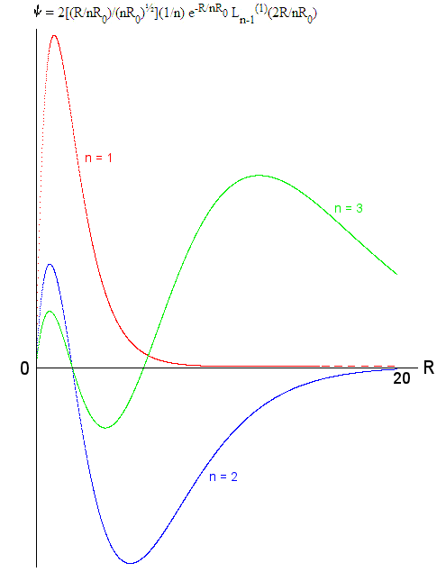
= nLp would be the radius of curvature as depicted in Figure 01a.
The commutative rule becomes : [t0 (dR/dt), R] = -i ,where t0 = tPl = (G /c5)½ = 5.4x10-44 sec and dR/dt = (-i/t0)d/dR so that[-i (d/dR), R] = -i . |
Figure 01d Probability Distribution |
2x1034, the spatial curvature would lower drastically to k
10-3 cm-2. Thus, the problem with the flatness of the universe can be explained as quantum jump to highly excited state. The transition to classic theory occurred naturally since such highly excited levels are crowded together like a continuum, where the discreteness characterized by quantum theory is lost. This theory has another virtue, e.g., the explosive expansion automatically stops with the end of the transition - unlike the original inflation theory, which requires a specific mechanism to have it terminated or it inflates forever creating endless universes. Last but not least of its novelty is the absence of the time variable in the formalism. It implies that the very early universe is timeless. The dynamics is driven by the dimension-less scale factor R.
4.6x10⁻²⁷ for Rb
2x1034. The averaged quantum fluctuation (carried over from the quantum era) of the scale factor |
Ra| would not be larger than Ra, thus |
Ra|
Ra
4.6x10⁻²⁷ <
T/T
10-5, which is at least consistent with the observation.
E
t =
with
E
1092 erg (from the energy density at inflation and the expanded volume). Consequently, the velocity of expansion v
rbRb/
t
10120 cm/sec >> c.![]() |
G) 10113 ergs/cm3 in agreement with the estimated energy infusion at the beginning of the universe (Figure 01f). While the cosmological constant term in the Friedmann Equation is considered to be negligible as the current estimate for the value of 10-56 cm-2 is very small, and it is supposed to be constant throughout the history of the post-inflation universe. See a 2015 update on "Vacuum Energy Density", and also "Composition of Early Universe".
|
Figure 01f Energy Density Evolution |
-only)
-only homogeneous and isotropic universe is rather problematic as shown below. Anyway, for those who don't mind the mathematical detail, it starts from the classical form :
R2/3)c2 = 0 --------- (10)
is the cosmological constant, k is the curvature of space, t the comoving time, and R the dimension-less scale factor.
, we can assign R to take the place of x and construct an entity having the dimension of ergs-sec = gm-cm2/sec (the dimension of
) such as (c2L3/G)dR/dt, where L is the linear size of the early universe. Thus the commutative rule becomes:
, which can be satisfied with (c2L3/G)dR/dt = -i
d/dR, or dR/dt = -i
(G/c2L3)d/dR ---------- (11).![]() |
![]() |
|
Figure 01h Quantum Harmonic Oscillator [view large image] |
Figure 01i Hermite Polynomials |
![]() |
![]() |
The eigenvalue and eigenfunction for the quantum harmonic oscillator is respectively : En = (n + 1/2) ![]() ---------- (13a), n = (m /![]() )1/4(2nn!)-1/2Hn(y)e-y2 ---------- (13b),where y = (m / )1/2, 2 = 
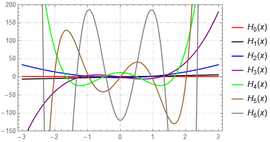
/m, and Hn(y) is the Hermit Polynomials (see Figures 01h, 01i).The corresponding solutions to the quantum empty universe's are : kn = k = -|k| = -(n + 1/2)(2/a0r0) ---------- (14a), n = (1/ a0r0)1/4(2nn!)-1/2Hn[(r0/a0)1/2 R]e-(r0/a0)R2 ---------- (14b) |
Figure 01j Pseudo-sphere |
If the initial size of the universe L and (3/| |)1/2 are taken to be the Planck length LP = (G /c3)1/2 = 1.62x10⁻³³ cm, then r0 ~ a0 ~ LP, the expressions assume the simple forms : |
n = (1/
LP2)1/4(2nn!)-1/2Hn(R)e-R2 ---------- (15b),
= |
|c4/(8
G) = 5.4x10113 erg/cm3, which is very close to the controversial vacuum energy density calculated for the purported dark energy.
|2 can be interpreted as the probability at certain value of the scale factor R for the universe. For example at ground state n = 0, R = 0 is the most probable configuration, i.e., the universe is most probable to be nothing.
= -|
| and k = -1 is :
|/3)1/2. For the current epoch
~ 10-56, the oscillating period T = 2
/H ~ 100 Gyr or tmax = T/4 ~ 25 Gyr, i.e., it is compatible with the cosmic age even though the other parameters do not seem to be quite right.
. Other than that, the quantized Friedmann Equation is essentially in the same form as Eq.(12a) differing by a factor of R2 in the 2nd term, that is :
/dR2 - V(R)
= 0 ---------- (16a),![]() |
![]() |
|
Figure 01k |
Figure 01l |
Actaully, the formulation has a serious conceptual problem, here's the comments : |
(R0/2) eHt for t
, i.e., the universe expands forever leading to "Big Chill" which may not be a problem.
-only universe. The case for k = +1 cm-2 is a rather contrived scheme. It really doesn't represents the quantum universe as it implies a linear size of 1 cm, for which any subject would be outside the quantum domain. On the contrary, in classical cosmology, the value of curvature has been arbitrarily assigned a number without much problem especially when the universe (since the inflationary period) is observed to have a curvature ~ 0 (see Planck).
/dR2 + v0R4
= 0 ---------- (19a),
= A cos{[(v0)1/2/3]R3} ---------- (19b),![]() |
|
Figure 01m Quantum Tunneling |
For the case of k = 0 cm-2, b0 = , P = 1, i.e., models of early universe with small curvature is free-range. |
![]() |
![]() |
|
Figure 02a Different Types of Solution |
Figure 02b Damped and Forced Oscillation |
(t). As it will be shown in the followings, this is the inflaton that drives the inflation and later on becomes the Higgs field endowing mass to all particles (see "Could the Higgs Boson be the Inflaton?"). It can be shown (see for example "Early Universe") that the energy density
and the pressure p associated with the scalar field can be expressed in the form (in natural units):
![]() |
![]() |
|
Figure 03a Inflaton Potential |
Figure 03b Inflaton Field |
![]() |
) = (1/2)m2
2 + (
/4!)
4, in which m2 is negative for endowing mass to particles (see "Spontaneous Symmetry Breaking").
= 0. The scalar field
has been solved numerically using this form of potential with a little push (small d
/dt) in the beginning to start the process. The result shown in Figure 03b is not quite satisfactory as it reaches the steady state too soon. A more realistic scenario is shown in the inserts (Figure 03a), in which the potential falls off much more gently allowing a slow-roll to the true vacuum. Note that the general form of
is similar to the damped oscillation with a constant force in Figure 02b.
(blue), and pressure p (black) as functions of the time t. It shows that the inflaton energy density and pressure vanish as it settles down to the true vacuum. The inflaton energy is converted to the particles in this world, while the negative pressure is responsible for driving the exponential expansion in this phase.
G)1/2 is the reduced Planck mass, and
o is the total mass density of the system in Planck scale (= 5x1093 gm/cm3), which is related to Vo =
oc2 = 10114 erg/cm3. It remains to be a constant during the exchange of energy between the inflaton's and particles' until the end of the inflation (see Figure 01f). Thus according to this scenario the early exponential expansion depends on the value of H = c(
/3)1/2 = (
o/3Mp2)1/2 = constant
2.6x1043 sec-1. Ultimately, the inflation is caused by the constant energy density Vo during that period. (see the simple mathematics to demonstrate the effect of constant energy density on gravitational force). During this period, the cosmological constant
=2.3 1066 cm-2, i.e., a 10123 folds difference from the value in the current epoch. See a 2015 update on "Vacuum Energy Density".![]() |
Eternal inflation is a peculiar property arising from the concept of inflation. The above-mentioned scenario is for just one point in space. It has been suggested that every point in the space can be initially in a false vacuum state. The decay to true vacuum happens randomly similar to the decay of radioactive substance. The difference is the continuously growing of the false vacuum (FV). As depicted in Figure 04b, the FV itself inflates continuously getting bigger and bigger (cannot be shown in the drawing). Those decayed regions are the "pocket universe" like ours, which keeps on expanding but not in exponential rate. |
Figure 04b Eternal Inflation [view large image] |
The chaotic inflation proposes that false vacuum with sufficient high energy density can pop up randomly within the the normally expanding universe. Exploration of variations on the inflationary theme has produced many speculative "theories" such as extra-dimension, multiverse, many worlds, pre-BigBang, ... |
![]() |
About a year after the introduction of the theory of inflation without considering any quantum effect, it was realized that quantum fluctuations in the initial region could have a profound consequence as tiny imperfection would become huge defect with the cosmic expansion (Figure 05a). Since then theoretical calculations yield close agreements with observations in the forms of CMBR power spectrum and super-clusters structures. The basic assumptions, the different kinds of spectrum, the link of gravitational potential fluctuations to the other types, and the evolution of the fluctuations to astronomical objects will be explored in the followings. In order to understand what it is all about, it is crucial to define the relationship between the fluctuation and power spectrum. |
Figure 05a Exponential Expansion [view large image] |
![]() |
![]() |
|
Figure 05b Fourier Transform |
Figure 05c Gaussian Distribution |
![]() |
2)/dk = A, the variance receives equal contributions from a given range of k. The gravitational potential fluctuation is said to be scale invariance as shown in Figure 05d. It is estimated that 
(x) is of the order 10-4 at kc = H and t = 1/H.![]() |
![]() |
![]()
|
Figure 05d Power Spectrum and Cosmic Fluctuations |
Figure 05e |
![]() |
![]() |
In Figure 05g the frozen waves are shown as if they are trapped under the "mountain" (it may take a moment to appreciate the contents as it plots everything inverse to length, i.e., inside out; contrary to the normal perception in the insert). As expansion of the universe continues, new particle waves are frozen on top of the previously ones. The process goes on until the end of the inflation when the universe already becomes populated by inhomogeneous fluctuations (see insert in Diagram a, Figure 05d). They become the source of mass-energy density |
Figure 05f Quantum Fluctuation |
Figure 05g Cosmic Horizon |
fluctuations (Diagram e) leading to gravitational fluctuations (Diagram d) and eventually the wall/void in super-galactic cluster and the temperature variations in the CMBR. |
![]() |
|
Figure 05h Formation of CMBR Spectrum and Cosmic Large Structures [view large image] |
See "Power Spectrum" and "Hubble Constant and 2018 Update" for more info about the formation of CMBR. |
![]() |
measurement related to the left of the "mountain" in Figure 05g. In order to prevent runaway gravitational fluctuation, it is believed that P(k) 
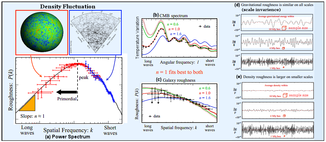
k for the mass density spectrum (Figure 05i). Subsequent interaction with the cold dark matter bends the curve as shown in Figure 05i. The large scale structures are in simpler form since there is no radiation to counteract the gravity. Although the CMBR spectrum also follows this scenario (Figure 05d, diagram a), its more complicated shape can be explained by further modifications (see "CMBR Power Spectrum").
|
Figure 05i Power Spectrum, Evolution [view large image] |
A rough estimate of the thickness of the "Last Scattering Shell" (Figure 05h) : For ne ~ 103cm-3 (from Figure 01f), scatter = 6.65x10⁻²⁵cm2; ~ 1021cm - about 10-2 times the observable cosmic size of 1023cm at recombination (see "History of the Universe"). |
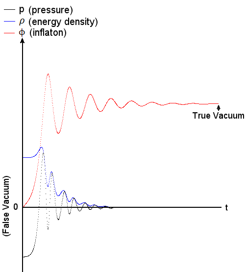
generated in the early universe. It turns out that both of them obey the same equation for the 
k. The tensor power spectrum has the form : P(k) = (8/MP2)(H/2
)2 implying low-energy inflation would
![]() |
produce negligible amounts of gravitational waves. No primordial or any other forms of gravitational wave has been detected so far (up until 2014). However, indirect evidence has been observed in the B-mode polarization imprinted on the CMB (to be confirmed by further evaluations). As shown in Figure 05j, the B-mode polarization is subjected to contamination by many effects in the intervening space before its detection on Earth making its confirmation very difficult. |
Figure 05j B-mode from Gravitational Wave |


see this illustration on separation of various theories. AND :