Harmonic Oscillator

Contents

Applications

The physics of Harmonic Oscillator is the second basic ingredient of quantum mechanics after the spinning qubits (see "Entanglement and Teleportation"). It introduces the concept of potential and interaction which are applicable to many systems. Its solutions are in closed form which enables relatively easy visualization. The usefulness is derived from the Taylor expansion of any function including the potential energy curve : The second term with the first derivative tends to vanish near the minimum of any function, while the first term is a constant which would not affect the physics. Thus, only the quadruple term survives with the other terms being negligibly small and this is precisely the form for the potential energy of the harmonic oscillator.

Figure 01a Diatomic Potential [view large image]

The force F = -dV(x)/dx = -k(x-x0), where k =[d2V/dx2]x=x0 .

Followings are some examples to illustrate the scope of its applications from classical to quantum physics.


• Hooke's Law - This is the classical example involving mass motion by spring. The solution is exact and simple, but provides all the basic ingredient in mathematical physics. The extension to forced and damping vibrations has even wider application in electrical and mechanical systems.


• Molecular Potential - The diatomic potential curve (Figure 01a) near its minimum is a good example of harmonic oscillator approximation.


• Coupled Oscillators - This system introduces the concept of eigenvalues and eigenvectors at the level of classical physics. The normal modes describe coherent motion of atoms in molecule and in crystal lattice.


• Quantum Field Theory - Imitating system of free harmonic oscillators to provide the basic concept for the quantization of field.

Classical Harmonic Oscillator

	According to the Newtonian mechanics, the equation of motion for this system is :
Figure 02a Classical Harmonic Motion [view large image]

Figure 01 Different Types of Solution [view large image]	Figure 02 Damped and Forced Oscillation [view large image]	In the above equation ks = (k/m)1/2 = , kd has unit sec-1.

Translatory Motion	Rotational Motion	Electric Circuit
Mass, m	Moment of inertia, I	Inductance, L
Stiffness, ks	Torsional stiffness, ks	1/Capacitance, 1/C
Damping, kd	Torsional damping, kd	Resistance, R
Impressed force, F(t)	Impressed torque, T(t)	Impressed voltage, V(t)
Displacement, y	Angular displacement,	Condenser charge, q
Velocity, v = dy/dt	Angular velocity, = d/dt	Current, i = dq/dt

Table 01 Types of Damped and Forced Harmonic Motion

Coupled Harmonic Oscillators

	The simplest coupled harmonic motion has two equal mass bodies linked by three identical springs as shown in Figure 03, where the edge points are fixed and the surface is friction-less. The equations of motion for this system are :
Figure 03 Coupled Harmonic Motion [view large image]

		translational motion, and another 3 for rotational (2 for diatomic, since there is no rotation around the inter-nuclear axis; and all such motions run as a whole). Figure 04 shows the only vibrational mode for the diatomic HCl molecule. According to a theorem in two-body problem, the motion can be reduced to a one body equivalence by using the reduced mass mM/(m+M) for one of the bodies while the other remains stationary. Figure 05 shows three vibrational modes for the tri-atomic molecule H2O. The even more complicated case can be found in crystal lattice.
Figure 04 HCl Normal Modes	Figure 05 H2O Normal Modes [view large image]

Quantum Harmonic Oscillator

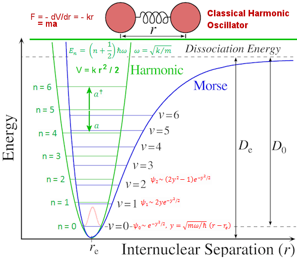
Instead of using the force to describe the dynameics of the system as in Newtonian mechanics, quantum mechanics is usually prescribed by energy (i.e., in the form of the Hamiltonian H = p2/2m + m2x2/2, where p = -i d/dx, and 2 = k/m) in the Schrodinger equation Hn = Enn. The eigen value (energy level) is En = (n + 1/2) . The zero point energy /2 usually is subtracted from the formula to avoid infinite energy in the vacuum. The wave functions can be expressed in terms of the Hermite Polynomials Hn(x), i.e., n(x) = Cn e-x2Hn. The explicit forms for few low lying states are shown in Figure 06. The formulation of quantum harmonic motion is useful in studying the vibrational modes of molecules and

Figure 06 Quantum SHM Wave Functions [view large image]

crystal lattice. The example of diatomic molecule below describes the vibration of the nuclei by more realistic potential (than the harmonic oscillator) such as the Morse curve (Figure 07).

The Morse potential has three parameters De, a, and re to be determined largely by the distribution of the electron cloud (electronic configuration, see inserts in Figure 07). With the small mass of the electrons, the adjustment of the electrons to new configuration is much quicker than the heavier nuclear vibration of the atomic nuclei. This is the base for the "Born-Oppenheimer" approximation which separates the motion (and thus the wave functions) of the atomic nuclei and electrons. The assumption in turn leads to the "Franck-Condon" principle as illustrated in the following mathematical exposition. The electric dipole transition is the dominant effect of the interaction between the electrons in a molecule with the electromagnetic field. In perturbation theory, the transition probability amplitude from an initial state to a final state ' is in the form :

Figure 07 Diatomic Molecule

Harmonic Oscillators and Quantization of Field

		space. Figure 08 shows the formulas and pictorially illustrates that a jumbled function in x-space can be decomposed into simple components in k-space. As dictated by the uncertainty principle, these 2 spaces are complementary to each others. A sharp peak in k-space means widespread plane wave. A wave packet would contain some extension in k-space (Figure 09). Such tool is essential in the development of quantum field theory.
Figure 08 Fourier Transform	Figure 09 Wave Packet [view large image]	Similarly, the position and number eigenvectors n(x), and | n can be switched between each other in terms of the bra-ket notations in the Hilbert space such that :

The description of field is entirely classical up to this point. The a(k)'s are just the amplitudes in the k-space of the Fourier transform. They are related to the porportions of various plane waves (in state k, and sometimes referred to as quantum waves) within the superposition. Quantization starts with the uncertainty principle which dictates the communitative relation [x, p] = i for a single particle. For the classical field, x is replaced by the field , while the conjugate momentum = /t is similar to the velocity v in p = mv. By these definitions, the equal time commutative relations are :

The similarity between the harmonic oscillators and quantum field operators is merely formal. Physically, there are no harmonic oscillators associated with the quantum field. The superficial similarity breaks down for coupled harmonic oscillators and more complicated field or the dynamics involved strong interaction.

For fermion field, quantization is accomplished via the equal-time anti-commutative relation between the field and its conjugate, e.g., {_i(x, t), _j(y, t)} = _i(x, t) _j(y, t) + _j(y, t) _i(x, t) = (x-y)_ij .

Since one of the communitative relations for boson #1 and #2 in state k is in the form a(k₁)a(k₂) = a(k₂)a(k₁). It can be shown readily that |k₁,k₂ = |k₂,k₁, which implies the 2 bosons are indistinguishable and hence both can be in a same state at one spot simultaneously. There would be a change in sign for fermions because of the anti-communitative relations, thus they are distinguishable. Each kind of particles is governed by different statistical formula as the consequence - the Bose-Einstein distribution for bosons and Fermi-Dirac distribution for fermions (see "Statistics"). This difference in statistical distribution

leads to different behavior. While Fermi-Dirac statistics is a crucially important concept for the understanding of the electrical and thermal properties of solids (see "Band Theory, Metal") on the assumption that metals contain free electrons similar to perfect gas (known as electron gas, Figure 10b). The Bose-Einstein statistics exhibits a very special property at very low temperature in the form of Bose-Einstein Condensate (BEC, see "Superfluidity"), where most of the bosons merge together as a coherent whole (see Figure 10a, 1nK = 10-9 K).

Figure 10 Quantum Statistics [view large image]

BTW, magnetic traps are techniques to drive hotter constituents from the confinement.