Quantum Field and 2nd Quantization (2021 Edition)

Contents

Quantum Field

		There is another level of quantum theory over the particle and wave as mentioned on "1st Quantization". In the Standard Model (SM) of elementary particles, it is the quantum fields that are ubiquitous in the formulation. In contrary to the classical fields such as the electro-magnetic fields in Maxwell's equations and the metric tensors in General Relativity, in which there is always a source such as charge and current or mass-energy tensor to generate the fields, the quantum fields in SM has no source - it is assumed to be everywhere and at all time in this Universe.
Figure 01 Quantum Fields [view large image]	Figure 02 Virtual Particles [view large image]	That's why there is always a suspicion about an even deeper level to describe the detail of their origin. See "Quantum Fields and Vacuum Energy Density" for more on vacuum state.

		vacuum, all its energy was converted to the particles in this world. Since then, there is the Higgs field, which also existed in false vacuum state and then settled down to the true vacuum level of 125 Gev above the zero point energy. It permeats throughout the universe uniformly and isotropically, and endows mass to other particles. The interactions between the particles and the Higgs maintain a meta-stable state which could end anytime according to one calculation (see "Stability of the Universe").
Figure 03a The 24 Quantum Fields	Figure 03b Elementary Interaction [view large image]	Figure 03a lists the 24 elementary particles (or quantum fields) in the Standard Model (should add the Higgs hoson discovered in 2012), while Figure 03b specifies the kinds of interactions by these particles.

There are 12 fermion and 12 boson fields in the Standard Model (Figure 03a). The Lagranian L for leptons is shown in Figure 04. It contains all the lepton fields (waves) and the interactions between these fermions and bosons. The Lagranian L1 contains 1 EM , 2 weak boson fields; L2 has 6 leptonic fermion fields; L3 is for the Higgs boson. At this level, we are dealing with waves excited from the underlaying fields, i.e., one step up from the more or less featureless elements (see Figure 01). The interaction is expressed in the covariant derivative D. There are altogether 3 coupling constants - g and g' are associated with the interaction between the gauge bosons W and B and the Higgs respectively, Ge is the Yukawa coupling constant, which defines the interaction between the Higgs and the lepton. The first three terms in Eq.(41c) are responsible for generating the mass of the gauge bosons, while the last term takes care of the fermion mass.

Figure 04 Lepton Lagranian for WS Model of SM [view large image]

The quarks have a slightly different form of the Lagrangians by the title of quantum chromodynamics (QCD).

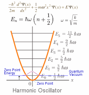
		Similar to the harmonic oscillator, each of these quantum fields has a zero point energy causing infinity in theoretical calculation. It is subtracted from the total by moving the zero point up as shown in Figure 04b. The energy density at the zero point level should be a constant and is often assumed to be the dark energy which accelerlates the cosmic expansion and becomes important in the recent epoch. The total is about 10-8 ergs/cm3 or 10-29 gm/cm3 (Figure 04c).
Figure 04b Zero Point Energy	Figure 04c Dark Energy Density

2nd Qunatization

-i(t-kx)

If a number operator Nk = ckck is defined such that it operates on the state vector |nk to generate: Nk|nk = nk|nk where nk is the number of particles in the k state; it follows that ck|nk = (nk+1)1/2|nk+1 ck|nk = nk1/2|nk-1 Thus ck increases the number of particles in the k state by 1, while ck reduces the number of particles in the k state by 1. They are called creation and annihilation operator respectively. The complete set of eigenvectors is given by:

Figure 05 Hilbert Space [view large image]

---------- (8) for all values of kl and nl. They form an abstract space called the Hilbert space (Figure 05) with all the eigenvectors orthogonal (perpendicular) to each other and the norm (length) equal to 1.

---------- (9)

Note that Eq.(11a) looks similar to Eq.(6) for the case of particle only. Closer examination reveals (x) = (x) indicateing that it really has no complex component.

There is another way to show the link between complex field and charge :

The symmetry of such invariance is related to the conservation of charge as shown in Eq.(11c), where the sum of N_c and N_d is a constant within a volume containing no source or sink. See further detail in "Lie Groups".

---------- (12)

---------- (13)

---------- (15b)

Interaction and Feynman Diagram

The formulation of free field quantization does not work anymore when interaction is included into the system :


• The commutation rule becomes very complicated. It is not even a c-number but a function of the field operators.
• It is not possible to construct states from the vacuum by applying the "interacting particle creation operators (certain form of c_k)".

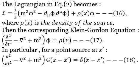
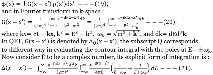
Figure 06 Green's Function [view large image]	G(x-x') is called the Green's function. It is the solution of Eq.(18) at the point source + free field otherwise. It is very useful in QFT.

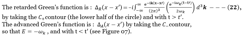
Figure 07 Contour Integral [view large image]

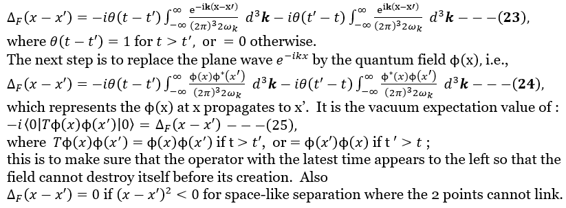
The Feynman Green's function (propagator) _F = _R + _A to take care of both particle and anti-particle respectively. Thus, :

Figure 08 Feynman Diagram [view large image]

The fermion-fermion scattering in Figure 08 will be used as an example to evaluate the corresponding S-matrix from the Feynman diagram (see also Table 03):


1. Collect the 4 quantum fields for the external fermion lines (_p1, '_p2, *_p3, '*_p4), plus other factors to be added later.
2. Multiply 2 coupling constants g₀ for each vertex.
3. Add a delta function (k - p₁ + p₃), or (k + p₂ - p₄) for the vertex x or x'.
4. Write down a propagator _F(k) for the internal line. It represents the virtual bosons for all values of the 4-momentum k.
5. Integrate over internal momenta. In explicit form :
   

In this case of tree diagram, the delta functions enforce the rule for energy-momentum conservation such that the internal momenta k = p1 - p3 = p4 - p2. Thus, the integration can be carried out trivially. Such is not the case for a loop diagram, which diverges quadratically (see for example the self-energy diagram in Figure 03f). The integration of the k-space yields: 1/[(p1 - p3)2 - m2] The S-matrix becomes : S = [(M/V)2(E1E3E'2E'4)-1/2] (*p3'*p4) {(g02)/[(p1 - p3)2 - m2]} (p1'p2) ----- (29), where M and Eps are the mass and energy of the fermions, V is the normalization volume. The scattering cross section is proportional to the squared S-matrix: |S|2.

Figure 09 Feynman and Friends [view large image]

Perturbation Theory

Figure 10a shows the Feynman diagrams corresponding to each term of the S-matrix expansion. The order number in S(n) is determined by the number of power in the coupling constant.

Figure 10a Higher Order Feynman Graphs [view large image]

f (Sfi)*Sfi = 1, which guarantees that probability is conserved in the process. Such relationship indicates that the matrix Sfi has an inverse, which in turn implies that it is possible to return to the initial state from the final state at least in principle although the probability is almost zero in practice so that the second law of thermodynamics is "almost" never violated. This property is also related to the conservation of information, which caused so much trouble for Stephen Hawking.

Figure 10b S-Matrix Elements [view large image]

Note: For example in the electron positron scattering process, there are three possible finally states as illustrated in Figure 10b. The sum of the probabilities for each one of these has to be: S*11S11 + S*21S21 + S*31S31 = 1 to insure the unitary condition.

Evolution of Quantum Fields

The 24 quantum fields as mentioned in the very beginning is not always like that according to modern cosmology (Figure 11).


1. Soon after Max Planck introduced the Planck constant h in 1899 to account for the spectrum of blackbody radiation, he realized that the only way to construct a unit of length out of h = 6.625x10^-27 erg-sec, the velocity of light c = 3x10¹⁰ cm/sec, and the gravitational constant G = 6.67x10^-8 cm³/sec²-gm, is L_PL = (Gh/c³)^1/2. This is the now famous Planck length.

   Subsequently, it transpires that the realm of Planck scale would involve entities with size of the order 10-33 cm and associated with high energy phenomena at 1019 Gev (see list below). Such environment is considered to occur at or near the moment of Big Bang - a most favorable theory for the creation of this universe. Here's the Planck scale :

   • Planck Length - L_PL = GM_PL/c² = (G/c³)^1/2 = 1.62x10^-33 cm.
   • Planck Time - t_PL = L_PL/c = (G/c⁵)^1/2 = 5.39x10^-44 sec.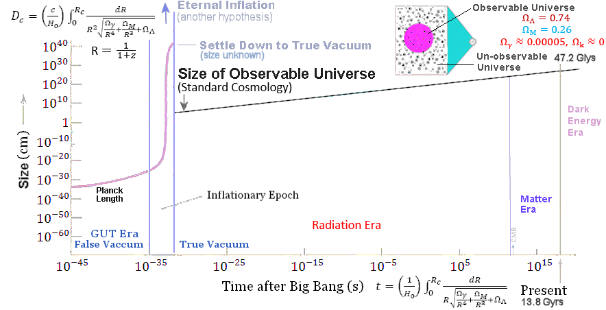

   		Planck Mass - MPL = (c/G)1/2 = 2.17x10-5 gm. Planck Energy - EPL = (c5/G)1/2 = 1.22x1019 Gev = 1.95x1016 erg. Planck Temperature - TPL = EPL/kB = (c5/GkB2)1/2 = 1.42x1032 oK. Planck Energy Density - PL = (c5/G2) ~ 10114 ergs/cm3.
   Figure 11 Modern Cosmology	Figure 12 Q Field Evolution	The Planck Era is the period before the Planck time of 5x10-44 sec. Not much is known; nevertheless, Quantum Gravity offers some haphazard guessing about this world of so-called "Realm of Planck Scale".

Actually, effort to formulate theory in time or size smaller than the Planck scale (~10^-45 sec, Figure 12) is doomed to fail as any system below such limit violates the uncertainty principle of t t_PL and x L_PL (for the corresponding Planck mass/energy) rendering it meaningless (see "What Is The Smallest Possible Distance In The Universe?").


2. The GUT Era (Figure 11) is the time interval from the Planck time of 5x10^-44 sec to the initiation of inflation at 10^-35 sec.

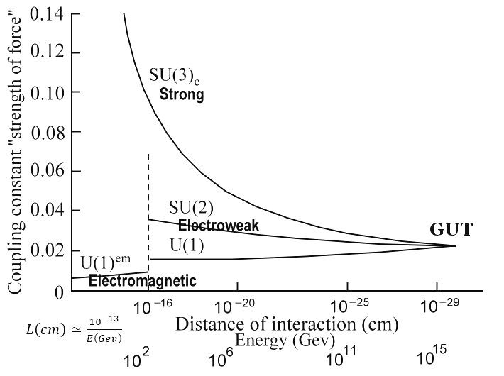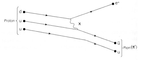
   According to the "Theory of Cosmic Inflation", there was an inflaton field in a state of false vacuum (Figure 13b) during this period. Also in co-existence were the gravitational field and one unified field (for the strong and electro-weak interactions, Figure 12). The Grand Unified Theory suggests that at energies above 1015 Gev, all gauge bosons can be produced freely and all interactions have the same strength (Figure 13a). The quarks can change color charges, as easily as transform into leptons (hence the proton decay, which failed to be confirmed experimentally leading to the desertion of the theory).

   Figure 13a GUT [view large image]

   See "Higgs Field, the Eternal and Ubiquitous (2021 Edition)"

3. The Era of Inflation lasted from 10^-35 to 10^-33 sec. At the end of inflation, the inflaton field dumped its excessive energy to create real particles as it decayed to the true vacuum in a process called "reheating" (see also "Cosmic Inflation and Reheating").
   The QCD fields for strong interaction split off soon after this period (Figure 12).
   According to SM, the Lagrangian for QCD is :

   In early universe up to 10-12 sec after BB, the fermions (u,d,s,c,b,t) are restmass-less, i.e., mi = 0. They couple to the SU(3) Gauge bosons Ga, (where the index "a" runs from 1 to 8) as well as the SU(2) Gauge bosons according to the Standard Model (see Figure 14). The system of quarks and gluons flew at the speed of light as some sort of fluid. This state of the QCD can be considered as free relativistic gas called Quark-Gluon Plasma (QGP, see "Quark-Gluon Plasma and the Early Universe").

   Figure 13b Inflation

   [view large image]

   		At 10-12 sec after BB (Figure 12), the electro-weak field split into weak and electromagnetic. The electroweak symmetry was broken at this time. The left-handed version of the fields behaves differently from the right-handed (see Lagrangians under Figure 14, or Figure 04). The em field split off on itself own becoming long range. This is the consequence of the
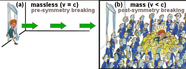
   Figure 14 SM, Parameters	Figure 15 Mass, Origin of [view large image]	Higgs field decay from its false vacuum state to the true vacuum endowing restmass to most particles. Before this event they all move at the speed of light (Figures 14, 15).

   Another phase change occurs about 10^-5 sec after BB. This one transforms the Quark-Gluon Plasma to the bound state of Hadons (see "Chiral Symmetry Breaking").
   
   

   	By taking into account the higher term of the SM (Standard Model) perturbation series, the vacuum potential of the Higgs field V is in the form :
   Figure 16 Stability of the Universe [view large image]	and the sum is over all SM particles acquiring a Higgs-dependent mass Mi. The precise form of V1 is not important in the present context, it just shows that the Higgs potential also depends on the particles it acts upon. Furthermore, only the heaviest top quark in the sum is retained in the following consideration.

   As shown in Figure 16,a and the above formula, the vacuum potential V depends on the mass of the Higgs m and also the mass of the top quark m_t. Computation of V with the various values of m and m_t yields different forms, which can be stable, meta-stable, or runaway (see Figure 16,a). Figure 16,b plots the result revealing our universe is possibly in an meta-stable state sitting on the verge of catastrophic decay into the true vacuum. The revelation produced sensational news headline around the globe one morning in 2013 (soon after the discovery of Higgs in July, 2012). A second wave of doomsday prophecy occurred in 2014 with Hawking's blessing on the revelation.