
| Home Page | Overview | Site Map | Index | Appendix | Illustration | About | Contact | Update | FAQ |
|
are employed to evaluate the physical properties. The followings use the Many-Body Schrodinger equation to illustrate how it is done to extract information about the many-body systems from individual atom to solid (Figure 01), then expanding to macroscopic systems and gravity. |
Figure 01 Many-Body System |
 |

|
Figure 02 Schrodinger Equation, Many-Body [view large image] |
See Figure 10 for a pictorial portrait of Ue(R). |

 |

|
Figure 03 Stationary Orbital |
See "An Introduction to Hartree-Fock Molecular Orbital Theory" for the original derivation, "Stationary-action principle", and "Lagrange multiplier". |
 |

|
Figure 04 H2 Molecular Orbitals [view large image] |

|


 |

|
Figure 05 Density Functional Theory (DFT) [view large image] |
There are two problems with this formulation : (1) It fails to incorporate the density n(r1) into the kinetic energy term Te. (2) It does not support the exchange energy Eex (the last term in Eq.(10b). |
 |

|
Figure 06 |
See "Figure 06, and Density of States, Fermi Energy and Energy Bands". |
 |

|
Figure 07 r and k Space of Lattice [view large image] |
See "Figure 07, and Solid State Physics" for Reciprocal Lattice. |
 |
Returning to the interacting electrons, it is assumed that the density dependence (in exponential power) is similar to the non-interacting case. Thus, according to Eqs. (10,a,b), (14) and (15b), the electron energy can be expressed as the functional of n : Ue[n] = VeN[n] + Te[n] + Vee[n] ---------- (16a) Similar to the HF Method, the DFT's ultimate task is to minimize Ue[n] together with the constraint P =  n(r)d3r - N = 0, i.e., n(r)d3r - N = 0, i.e., L[n] = 0 ---------- (16b), L[n] = 0 ---------- (16b),where L[n] = Ue[n] -  P[n] ---------- (16c). P[n] ---------- (16c).
|
Figure 08 Stationary |
See Figure 08. |
 (x,x') instead of n(r1)/N. The single electron coordinate r1 has split into x and x' to represent 2 opposite spin states and (x,x') becomes a matrix called "density matrix" (see "von Neumann Entropy").) is the quantum version of the "Shannon's Measure of Information" :
 i pilog2(pi), i.e.,) = -Tr[
 n()] ---------- (18),
 |

|
Figure 09 Entanglement and Ec [view large image] |
Entanglement Measure and EHF (and thus Ec from E.(17)) has been calculated for 10 Helium-like atoms, e.g., H-, He, ... Ne+8 as shown in Figure 09. It shows a definite correlation between the 2 entities (see original article on "Correlation energy as a measure of non locality") |
 |
 The second term with the first derivative tends to vanish near the minimum of any function, while the first term is a constant which would not affect the physics. Thus, only the quadruple term survives with the other terms being negligibly small and this is precisely the form for the potential energy of the harmonic oscillator. |
Figure 10 Potential Curve [view large image] |
Thus, Ue = k(R-Re)2/2, where k =[d2Ue/dR2]R=Re ---------- (20). |
 |
The Harmonic Oscillator Schrodinger equation H  n = (p2/2m + m n = (p2/2m + m 2x2/2)n = Enn ---------- (21), 2x2/2)n = Enn ---------- (21),where p = -i  d/dx, and 2 = k/m. The eigen value (energy level) is En = (n + 1/2) . The zero point energy /2 usually is subtracted from the formula to avoid infinite energy in the vacuum. The wave functions can be expressed in terms of the Hermite Polynomials Hn(x), i.e., n(x) = Cn e-x2Hn. The explicit forms for few low lying states are shown in Figure 11. The formulation of quantum harmonic motion is useful in studying the vibrational modes of molecules and crystal lattice. d/dx, and 2 = k/m. The eigen value (energy level) is En = (n + 1/2) . The zero point energy /2 usually is subtracted from the formula to avoid infinite energy in the vacuum. The wave functions can be expressed in terms of the Hermite Polynomials Hn(x), i.e., n(x) = Cn e-x2Hn. The explicit forms for few low lying states are shown in Figure 11. The formulation of quantum harmonic motion is useful in studying the vibrational modes of molecules and crystal lattice.
|
Figure 11 Quantum SHM Wave Functions [view large image] |
The Morse curve Ue = De[1 - e-a(R-Re)]2 ---------- (22) (see Figure 10,b) is a more realistic model, where De is the dissociation energy at R  , ,"a" determines the width of the curve, and Re is derivated from dUe/dR = 0. |
 |
In presenting the potential curve for a diatomic molecule, one of the atomic nuclei is usually fixed at the origin of the coordinate frame. The other nucleus is then portrayed as vibrating and rotating inside the potential well as shown in Figure 10. The vibration is restricted to discrete energy levels. Each of the vibrational energy level v is further split into a series of rotational energy levels J called vibrational band. When the Schrodinger equation of Eq.(21) is expressed in spherical coordinates, separation of the spatial variables and wave functions into Y(R),  ( ( ), and Z( ), and Z( ) turns it into 3 equations : ) turns it into 3 equations :
|
Figure 12 Energy Levels |
 is called Spherical Harmonic. to a final state ' is in the form :
 v is the essence of the "Franck-Condon" principle. In layman's language, it states that the preferred transition occurs when the initial and final wave functions overlap more significantly. This condition is satisfied most often at the turning points, where the momentum is zero as shown by the (blue, green) transition arrows in Figure 10,b).
 1 at a time. Mathematically, it is the transition probability in Eq.(25) that determines whether a transition would occur. Here's a simple example of transition induced by the z-component of
  e, i.e., z = e cos() :
 v = 1. The electronic selection rule should abide to those for rotation, vibration, plus total spin S = 0. See Figure 12b, "Selection Rules" and "Selection rules and transition moment integral".
 |
About 80% of the free elements at room temperature exists in the form of metal. The conditions to form metal are vacant valence orbitals and low ionization energies. Similar to the splitting of energy levels when two or more atoms come close to each other; (See Figure 04.) energy levels broadened to a band (many closely spaced energy levels) for an aggregate of many atoms as shown in Figure 13,a. |
Figure 13 Band Theory |
See "Solid State Physics". |
| Due to the "Exclusion Principle" or equivalently the "Fermi-Dirac statistics", the valence electrons from the sodium atoms cannot occupy the same energy level of each others, they fill up the energy bands up to half of the 3s band at 0K (because the 3s level is only half filled, it can accommodate 2 electrons but there's only 1 in sodium atom), at an energy called Fermi energy EF. Figure 13,b shows that if there is empty levels available in the energy band, the valence electrons will be able to roam among the space in between the atoms by absorbing energy from the environment when the temperature is above 0K. With a few exceptions, metals have a silvery-white color because they reflect all frequencies of light. They have high electrical and thermal conductivity and all metals can be drawn into wires or hammered into sheets without shattering, i.e., they are ductile and malleable. These attributes are | the result of mobile, non-rigid electron gas within the lattice. Most metals (except gold, silver, platinum, and diamond) do not occur as free elements in the Earth's crust. They are usually found in chemical combination with other elements as mineral ores. Figure 13,b also shows that in an insulator, the valence band is full and the next empty energy band is separated by a large energy gap. Conduction cannot occur unless some of the electrons in the valence band are promoted to the conduction band. Energy needed to promote a few electrons might be provided by heating the solid to a very high temperature or by shining X rays on it. No solid can remain a good insulator while it is exposed to X rays. A semi-conductor has a smaller energy gap. Electrons can be promoted to the conduction band as a result of irradiation such as the conversion of sunlight to electricity by means of a silicon cell. |
 |
 |
The formation of band structure as shown in Figure 13,a is based on the model of "Free Electrons". Actually, there are atomic nuclei, which is characterized by periodic separation "a" with a corresponding potential VG(r) = VG(r+a). As shown in Figure 13,c and its magnifying version in Figure 14, for most values of the variable k = 2 /, the electron energy E0 = 2k2/2me. Only at k = n/a, the energy splits to EG = E0 VG(k), where VG(k) is the Fourier transform of VG(r). This is the origin of the "Band Gap". /, the electron energy E0 = 2k2/2me. Only at k = n/a, the energy splits to EG = E0 VG(k), where VG(k) is the Fourier transform of VG(r). This is the origin of the "Band Gap".
|
Figure 14 Band Gap [view large image] |
Figure 15 Semiconductor Doping [view large image] |
However, the band gap can be altered by in-purity doping which has the effect of narrowing the band gap as shown in Figure 15 either by adding electrons or introducing holes in the conduction band. This is the idea of semi-conductor. |
 |
Plasma is the fourth state of matter in which the components of the atom become separated. It is not produced by phase change. Its production depends on the separation of the atomic nuclei and electrons. Once detached, they move around independently and form a globally neutral mixture. Plasma is found in the stars and the interstellar environment making up most of our universe (~ 99 %, = 100% in early universe) under a wide range of temperature and density (Figure 16a). However, such condition does not occur frequently on Earth and that's why life can exists here. In our everyday life, plasmas have many applications (including nuclear-fusion, micro-electronics, television flat screens and so on), of which the commonest is the neon tube. The Schrodinger equation is useless in describing the dynamics of plasma. The equations of motion are prescribed by the "Navier-Stokes Equations" in fluid dynamics. |
Figure 16a Plasma Physica |
 |
as input parameters or established facts from the theory for the higher (larger size) level. Details in the lower level can be neglected by the theories for higher levels (such methodology is called "Effective Theory"). Figure 16b illustrates some of the systems according to the size of their components. The classification is incomplete as there are many more systems below, above, and in between. |
Figure 16b Reductionist's Systems [view large image] |
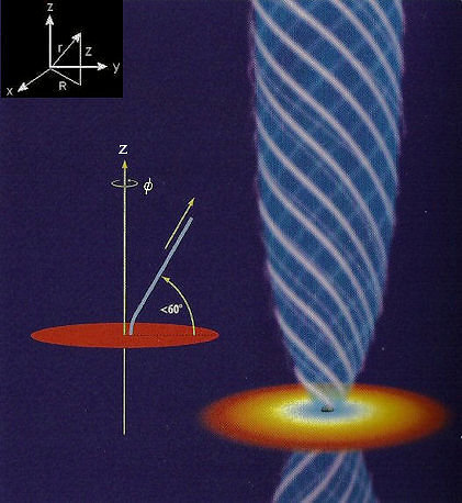 |
Nobody has seen a black hole until the silhouette in M87, 2019. Nevertheless, schematic diagram such as the one shown in figure 16c invariably presents a system composed with a central object (the black hole), an accretion disk, and a pair of jets moving along twisted magnetic field lines. This picture of the black hole is based theoretically on the combination of three branches of physics - Fluid Dynamics, Electromagnetism, and Gravitation. The effect of gravity from the black hole is characterized by the escape velocity vesc(r) = (2GM/r)1/2, where M is the mass of the black hole, and r = (R2 + Z2)1/2 provides a link between the spherical and cylindrical coordinates (see upper left corner insert in Figure 16c). With the assumptions of infinite conductivity (for the plasma in the system), isotropic pressure, local charge neutrality, non-relativistic inter-particle speeds), the suite of MHD equations are : |
Figure 16c Black Hole Schematic [view large image] |

 |
|
Figure 16d MHD Computation |
= 30o with the rotation axis, protrude from the disk and through the corona initially. The lines are dragged along by rotation creating a B component. |
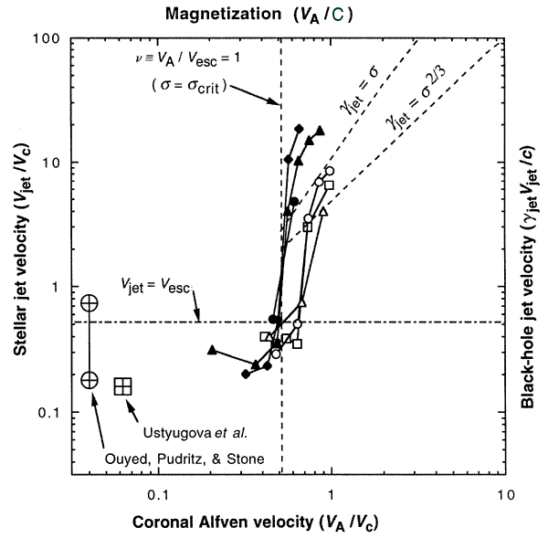 |
 = vA/vesc. The jet speed is low for < 1, i.e., for weak magnetic field (relative to gravity). The speed rises sharply when > 1. The ratio is therefore referred to as "magnetic switch" to turn on a pair of jets from a state with no jet. = vA/vesc. The jet speed is low for < 1, i.e., for weak magnetic field (relative to gravity). The speed rises sharply when > 1. The ratio is therefore referred to as "magnetic switch" to turn on a pair of jets from a state with no jet. |
Figure 16e Jet Switch |
rc = 2x1012 cm ~ 30 Rsun, while  = (1 - v2/c2)-1/2 is the Lorentz factor and = (1 - v2/c2)-1/2 is the Lorentz factor and  = 11(vA/c)2 for the black hole. The two dash lines are taken from the "Relativistic Wind Theory" which excludes the effect of gravity. = 11(vA/c)2 for the black hole. The two dash lines are taken from the "Relativistic Wind Theory" which excludes the effect of gravity. |
v, changing vesc to jet[2(1+vA2/c2)GM/r]1/2 etc. The quantitative difference is in the range of a factor of two or so. The qualitative conclusion remains the same.. However, it can be shown that if the displacement current term is retained in the Ampere's Law, the Alfven wave velocity becomes uA = vA/[1+(vA/c)2]1/2, which is reduced to uA ~ c for vA >> c, while uA ~ vA for vA << c. His work was not taken seriously until such wave was detected in the lab in the late 1950s. Eventually, he was awarded the Nobel prize for the efforts in 1970. |
Thermodynamics is a branch of physcis developed in the 19th century. It began with the invention of the steam engine (Figure 17) at the beginning of the industrial revolution. It was driven by the need to have a better source and more efficient use of energy than the competitors (among English, French, and German). It was a case where technology drove basic research rather than vice versa. Thermodynamics provides a macroscopic description of matter and energy. Today better insight is obtained by linking the subject with the statistical behavior of microscopic particles. They are gas molecules that can collide and possibly interact with each other. Since it's hard to exactly describe a real gas, it is often substituted by the Ideal gas as an approximation, in which the particles interact only by elastic collision, and take up no volume. |
Figure 17 Steam Engine [view large image] |
) have a specific value corresponding to that state. The values of these properties are a function of the state of the system. The number of properties that must be specified to describe the state of a given system (the number of degree of freedom) is given by Gibbs phase rule:  |
For example, the phase rule indicates that a single component system (c = 1) with only one phase (p = 1), such as liquid water, has 2 degrees of freedom (f = 1 - 1 + 2 = 2). For this case the degrees of freedom correspond to temperature and pressure, indicating that the system can exist in equilibrium for any arbitrary combination of temperature and pressure. However, if we allow the formation of a gas phase (then p = 2), there is only 1 degree of freedom. This means that at a given temperature, water in the gas phase will evaporate or condense until the corresponding equilibrium water vapor pressure is reached. It is no longer possible to arbitrarily fix both the temperature and the pressure, since the system will tend to move toward the equilibrium vapor pressure. For a single component with three phases (p = 3 -- gas, liquid, and solid) there are no degrees of freedom. Such a system is only possible at the temperature and pressure corresponding to the Triple point. |
Figure 18 Phase Diagram |
One of the main goals of Thermodynamics is to understand these relationships between the various state properties of a system. Equations of state are examples of some of these relationships such as the ideal gas law: |
 |
 |
In fact, it is these forces that result in the formation of liquids. By taking into accounts the attraction between molecules and their finite size (total volume of the gas is represented by the red square in Figure 19), a more realistic equation for the real gases known as van der Waals equation was derived way back in 1873 : |
Figure 19 Ideal Gas Modification |
Figure 20 Real Gas |
(P + an2/V2) (V - nb) = nRT ---------- (29a) where "a" is related to the interaction and "b" for the finite volume (see insert in Figure 19). Figure 20 lists these constants for some real gases. |
 |
 Eq.(30) looks formidable and the graphic is entangled (see Figure 21). However, there is one saving grace : the gravitational force is always attractive concentrating huge mass such as galaxies, stars, ... and the Earth. |
Figure 21 Newtonian Many-Body |
This disposition reduces the many-body "mumbo jumbo" to one single dominating force center under which everything moves, finer details could be added as perturbation. Here's a few examples to illustrate the usefulness of Newtonian mechanics over the last 400 years (see Figure 22). |
 |
|
Figure 22 Applications [view large image] |
The Many-Body problem in Eq.(30) is reduced to d2y/dt2 = g, the solution of which is y = gt2/2 + vt + h (see Figure 22,a) - the trajectory of a projectile. |
 |

|
Figure 23 |
as derived from Eq.(30), and see Figure 23. |
 |

|
Figure 24 Kepler's Three Law |
This is the Kepler's 1st Law. The 2nd Law is expressed by dA/dt = L/2m = constant, where dA = (r2/2)d. While the 3rd Law is covered by T = ab/(dA/dt) giving T2 = (42/GM)a3 (See Figures 24, and 22,b). |
 |
At the end of the 19th century, the French mathematician Henri Poincare tried to solve the differential equations for the three body problem. It was noticed that the orbit is not periodical anymore (in contrary to the case with just two bodies), actually the motion appears to be random. Then it was found that the solution is "exquisite sensitivity to initial conditions". The object would follow a very different path at the slightest change of initial condition. Figure 25 is an animation showing two paths of a third body under the gravitational influence of two massive objects. The paths start at the same position but the velocities differ by 1%. Initially the paths are very close, the difference becomes apparent after a while. |
Figure 25 3-Body System |
 |

|
Figure 26 Lagrangian Points [view large image] |
This is exactly the distance to L1 - the parking lot for many of the artificial satellites. However, it is known to be unstable, thruster burns manoeuvre is required to keep the object in place. |
 i mir'i = 0, r'i = constant, then the equations of motion can be written down in terms of the force F and torque T summing over all the particles in the system :
 |
 |

|
Figure 27a Rigid Body System |
Figure 27b Moment of Inertia |
The rotational term can be neglected if the size of the solid is much smaller than the distance scale. The object becomes a point mass without structure, either because it is so "small" or it can be represented by the Center of Mass. |
 |
 |
Earth when the spacecraft reaches hyperbolic excess velocity v  = (GM/|a|)1/2 (see Figure 28a - the hyperbolic curve), the flight can be switched to the heliocentric frame of reference (for both the velocity of the spacecraft relative to the Sun and the subsequent heliocentric orbit, see Figure 28b). = (GM/|a|)1/2 (see Figure 28a - the hyperbolic curve), the flight can be switched to the heliocentric frame of reference (for both the velocity of the spacecraft relative to the Sun and the subsequent heliocentric orbit, see Figure 28b).The total orbital energy E for mass m near the Earth is : E = mv2/2 - mGM/r = mGM/(2|a|) = constant > 0 ---------- (31). |
Figure 28a Conic Curves |
Figure 28b Reference Frames |
It is bound to the Earth for E < 0, free-run for E > 0, and just enough to escape for E = 0. See "specific orbital energy"  = E/m = GM/(2|a|) = constant. = E/m = GM/(2|a|) = constant.
|
 |
 |
|
Figure 29a |
Figure 29b Orbital Transfer |
treat the maneuver as an impulsive change in velocity while the position remains fixed. See "Cassini's Flight Path". |
 |
|
Figure 30 Space Flight [view large image] |
Figure 30,c is an example for landing on Mars (see detail). See a detailed guide on "Rocket and Space Technology", and a course lecture on "Celestial Mechanics". |
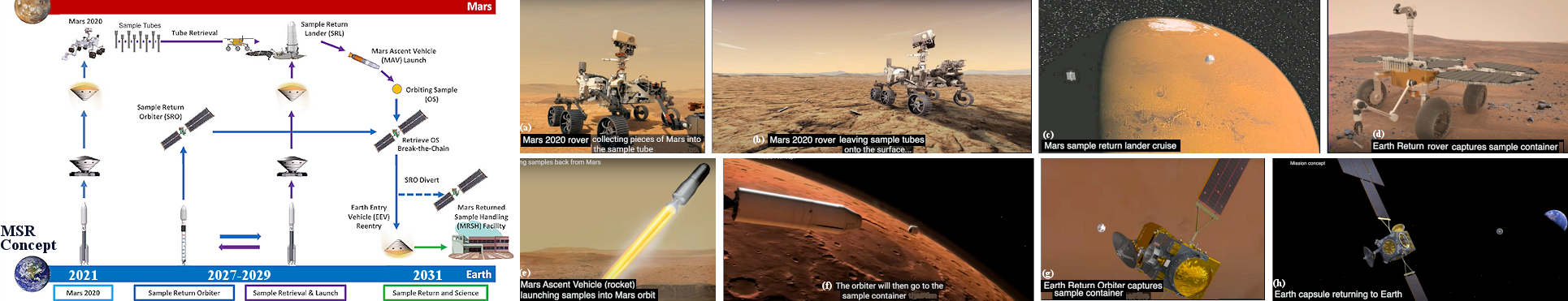 |
By early 21st century, technology has advanced to the point which enables the return of Mars sample to Earth. In April 2018, a letter of intent was signed by NASA and ESA that may provide a basis for a Mars sample-return mission. In July 2019, a mission architecture was proposed to return samples to Earth by 2031. |
Figure 31 MSR Concept [view large image] |
See "Summary of MSR (Mars Sample Return)" |
 Figure 32 Andromeda Strain [view large image]
