Monte Carlo Methods (2022 Edition)

Contents

Original Idea and Bernoulli Probability

The Monte Carlo Method was invented by Stanislaw Ulam (1909-1984). He was born in Poland and became a US citizen in 1941. During WWII, he was a team member of the Manhattan Project making nuclear bomb. In particular, he worked on the neutron diffusion problem in "gun-type" bomb. It leads him to further investigation of numerical computations for very complicated systems. With the newly availability of general-purpose electronic computer, he proposed a new way to estimate statistically the probability of a certain process. This is the original idea of Monte Carlo Method named in reference to his uncle's fondness for gambling in Casino Monte Carlo (Figure 01).

Figure 01 Monte Carlo Casino [view large image]

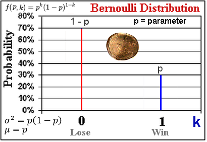	No mathematics is involved for checking biased coin, i.e., other than p = 1/2. The outcome is determined by just counting the numbers for p and (1-p). The counting should be done by computer since the accuracy depends on large number of countings. Once the process is completed, the skew can be estimated by the mean (p = 1/2 is fair) : The variance is :
Figure 02 MC with Bernoulli Distribution	For p = 0; k = 0, f(0,0) = 1 or k = 1, f(0,1) = 0 - the case for complete lose. For p = 1; k = 0, f(1,0) = 0 or k = 1, f(1,1) = 1 - the case for certain win. For p = 1/2; k = 0, f(1/2,0) = 1/2 or k = 1, f(1/2,1) = 1/2 - the case for fair play. N.B. f(p,0) + f(p,1) 1.

Random Probability Distribution

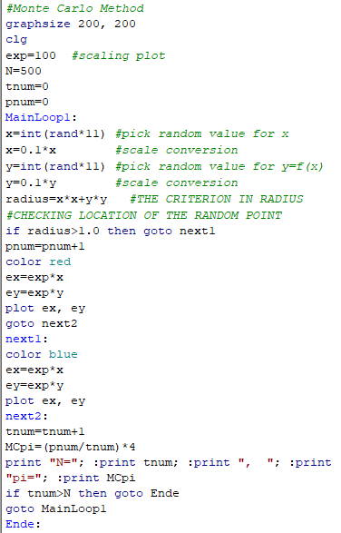
	The points are inserted randomly into the graph, accuracy depends on large number of points.
Figure 03 Monte Carlo with Random points	See "Table of Integrals".

		When the observed or measured data are arranged in an array . An algorithm similar to the one shown in Figure 05 is still workable if the checking of the random data (whether below or above the data point) is performed against the array. A curve from theoretical calculation or table by model simulation should have some sort of function available. An algorithm similar to the one shown in Figure 05 is again workable if the checking of the random data (whether below or above the data point) is performed against the curve or table (see lot of examples in "Power Spectrum").
Figure 04 DIY Monte Carlo	Figure 05 Algorithm	Finally, it can be resort to brute force by visual counting of the random points inside the intended area as shown by the square + isosceles triangle in Figure 06.

	The area under the irregular curve is A = (0.4x0.4) + (0.4x0.4)/2 = 0.24 . Visual counting obtains n = 35 points inside the area, the total number of points N = 5x9 = 45 giving the ratio r = n/N = 0.78. Since the total area is 0.4x0.8 = 0.32, A ~ 0.78x0.32 = 0.25 QED (See Figure 06).
Figure 06 MC for Irregular Function [view large image]	Indeed, the area under this shape can be computed with an array as suggested above producing the same value of A ~ 0.24 (See the corresponding algorithm).


The integral I in Eq.(4) can be expressed in term of the constant distribution function
(x_i) = 1/N with Then :

This alternative expression legalizes the "hand-waving" assertion stated earlier. It also introduces the concept of probability density distribution (x) = constant for this particular case. In general, it could be any function such as the "Binomial Distribution" shown by the red dotted area in Figure 08.

[Top]

---

Binomial and Gaussian Probabilities

The Bernoulli distribution in Eq.(1) specifies only one outcome with either win or loss. The binomial distribution provides further information about the chance of certain win/loss combination, e.g., p^N-k(1-p)^k in N trials. The distribution of each occurrence (the coefficient) is in the form :


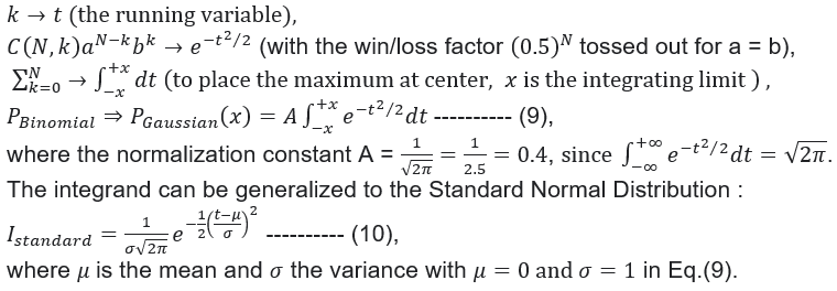
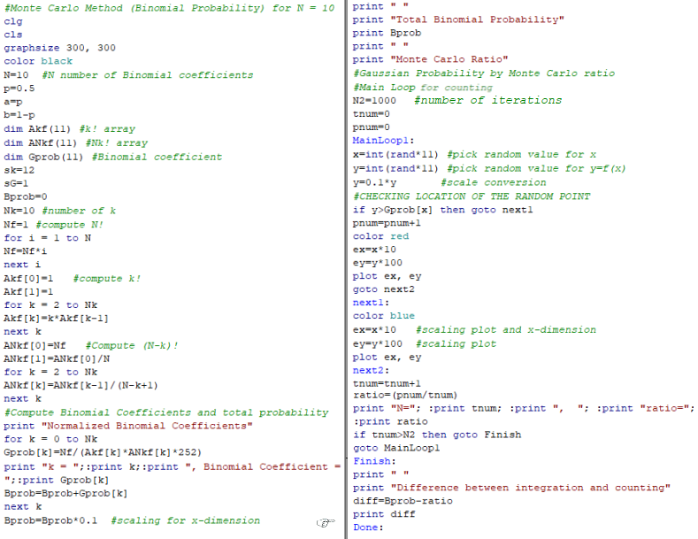
	C(N,k)=N!/[k!(N-k)!] ---------- (7), where the factorial q! = q(q-1)(q-2)...1, and 0! = 1 (see red dots in Figure 08, also see a "table"). The Binomial probability is defined by : PBinomial = (a + b)N = C(N,k)aN-kbk 1, ---------- (8) where a = p, b = (1 - p).
Figure 07 Binomial Distribution	In case a = b, it is called Gaussian or Normal probability PGaussian which is symmetrical with respect to its maximum. For a b, PBinomial reveals a skew from symmetry as shown in Figure 07 for p = 0.7. PBinomial goes-over to continuum as N with the following transitions :



As stated previously, the Monte Carlo (MC) method uses counting to estimate the area under a certain function. In principle, DIY MC can be done without any knowledge of calculus, simple arithmetic will do. In practice, the work is much easier by doing it with a computer algorithm using for example a free programming language such as Basic-256. Here's a simple Flow Chart :



See the "computer program" for detail. Essentially, the program scales the Binomial probability on an 1x1 square graph. Figure 08 shows the area under the probability curve in red. The counting ratio between the numbers under the curve and the whole square is : ratio = 0.4 similar to the area by numerical integration. This scaled value of total probability can be reverted to "1" with the multiplication of .

Figure 08 Binomial Probability by Monte Carlo


The Gaussian distribution can be considered as one of those probability density distributions (x) mentioned earlier. For example :


In general, the integrand can be very complicated and becomes more formidable by the addition of (x). Fortunately, many standard distributions are available in the form of "subroutines" for public use (at a fee). For example, with f(x) = x2, it can be evaluated using 1/2 of the array for the Binomial distribution from the previous examples. Figure 09 shows the integrand obtained by the Monte Carlo method in few red dots (see "computer program" + scaling ). The solid curves are evaluated by conventional method for comparison. Integration can be performed by the Monte Carlo method as usual if each piece of the integrand is stored in another array.

Figure 09 Find Integrand with Probability Density by Monte Carlo [view large image]

Essentially, the program picks a random value of x by which f(x) is multiplied to (x). The integrand is evaluated as f(x)(x). A corresponding curve would emerge in a plot with increasing number of iterations, or by just running the x index from xi to xf (5 to 10 here).




[Top]

---

Generalization

The "Bivariate Normal Distribution" is a simple introduction into the multi-variate cases. It just adds one more running variable

		together with another normal distribution (un-correlated) into the process (see an example in a "computer program"). Figure 10 shows the result pictorially in a 3-D graph (no such convenience beyond the bivariate). The newly created normal distribution can be stored in another array for further processing, but the size of the array and computer time rapidly become un-manageable as the number of dimension increases.
Figure 10 Bivariate Distribution	Figure 11 MC Generalization	Assuming unlimited computing resources, there is no problem extending the procedure to multivariate functions (dimension > 2). As shown in Figure 11, the probability density distribution (x1,x2,...) can be in various forms to generate f(), then goes on to produce the integral of the whole thing.

Note that f() is similar to f(x)(x) in previous notation, (x) is the known density distribution, while f(x) is an arbitrary function.

[Top]

---

Bayesian Monte Carlo

	Bayesian Theorem - It introduces a new kind of probability P(H|D), which relates the probability of "event H" given that "event D" has taken place. As shown in Figure 12, P(H|D) = [P(D|H) x P(H)] / P(D) ---------- (11), where P(H) and P(D) are the probabilities of observing H and D independent of each other.
Figure 12 Bayesian Probability	Actually, it is somewhat mislabelled for the event H as "Hypotheses" (which causes so much distress for Calvin the comic character, see insert in Figure 12), and D as "Data".

The neutral noatations would be just events A and B.
P(A|B) is the probability of event A given the occurrence (appearance) of B such that
P(A|B) = [P(B|A) x P(A)] / P(B) ---------- (12A),
or vice versa : P(B|A) = [P(A|B) x P(B)] / P(A) ---------- (12B),
and also [P(A|B) x P(B)] = [P(B|A) x P(A)] ---------- (12C),
i.e., the correlated probabilities are the same by taking into account the frequency of independent appearance (in %).
The correlated probabilities would be zero if the 2 events are not related.

Here's an example to find out the probability of fire (A) if there is smoke (B), i.e., P(A|B).


	From available statistical data, probability of smoke without fire P(B) ~ 50%, i.e., rather common and fire without smoke P(A) ~ 1%, i.e., very rare. Giving that the probability of smoke with the apperence of fire is almost certain P(B|A) ~ 99%, P(A|B) = [P(B|A) x P(A)] / P(B) = (0.99 x 0.01) / 0.5 ~ 2%.
Figure 13 Smoke and Fire [view large image]	Lastly, the correlated probability (plus) [P(A|B) x P(B)] = [P(B|A) x P(A)] ~ 1%, with the appearance of either fire or smoke.

Since the probability P(A|B) 1 by definition (actually for any probability), in this special case of P(B|A) ~ 1, violation occurs if P(A) > P(B); then we would live in a weird world of more fire than smoke.



Figure 14 Bayesian Monte Carlo

See "Simple Monte Carlo", and "Bayesian Monte Carlo" for more details.