Quantum Computing

Qubit and Entanglement
Quantum Logic Processing
Factoring and Encryption
Searching
Error Correction
Quantum Computing with Discord
Teleportation

Qubit and Entanglement

Physics and Computer science have combined to create a new field: quantum computing and quantum information. The spark that ignited world wide interest in this new field sprang forth in 1994 with Peter Shor's discovery of a theoretical way to use quantum mechanical resources to unravel a mathematical problem at the heart of electronic commerce and cryptography.

Basic steps towards the creation of a quantum computer have been taken, with the demonstrations of elementary data storage and manipulation using photons and atoms or trapped ions as the quantum bits, or "qubits". Recently, it has been shown that it is possible to build solid-state qubits made from tiny samples of superconducting material. Figure 01 shows some of the subjects, which are currently being investigated in the field of quantum computing.

Figure 01 Qunatum Computing [view large image]

It must be scalable: it needs a set of qubits that can be added to indefinitely.
It must be possible to set all of the qubits to a simple initial state, such as all 0.
The interactions between qubits must be controllable enough to make quantum logic gates.
To perform operations using these gates, the decoherence times must be much longer than the gate-operation time (typically milliseconds to seconds).
There must be some readout capability.
To link up the computer's circuitry, it must be possible to convert memory qubits into processing qubits, and vice versa.
It must be possible to move processing qubits accurately between specified locations.

Qunatum computing exploits two resources offered by the laws of quantum mechanics: the principle of superposition of states and the concept of entanglement. Superposition is a "one-particle" property; while entanglement is a characteristic of two or more particles.

Consider a particle with spin such as the electron. With reference to a given axis (say along the z axis), the spin of the particle can point in two opposite directions, say "up" or "down", and the spin states can be denoted as |1

and |0

. But by the laws of quantum mechanics, the particle can exist in a superposition of these two states (or wave of probability), corresponding to arbitrary orientation as shown in Figure 02.

Figure 02 Qubit [view large image]

Mathematically, the superposition of these two states can be written as:
|f

= a |1

+ b |0

------ (1)
where a and b are related to the probability of finding the electron in state |1

and |0

respectively satisfying
|a|² + |b|² = 1. This normalization defines the total probability of finding the electron to be 1. In general, the
|1

and |0

states can be represented by any two-states entity such as "on" and "off", horizontal and vertical polarization of a photon, one particle vs no particle, ... etc.

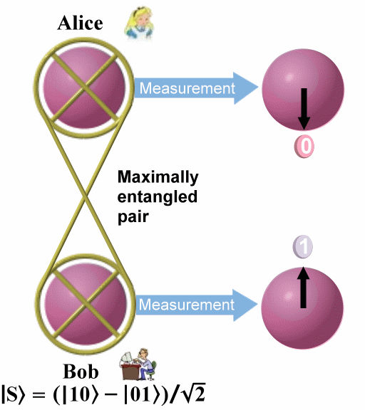
is called a qubit. If a photon in state |f

passes through a polarizing beamsplitter -- a device that reflects (or transmits) horizontally (or vertically) polarized photons -- it will be found in the reflected (or transmitted) beam with probability |a|² (or |b|²). Then the general state |f

has been projected either onto |1

or onto |0

by the action of the measurement (sometimes it is referred as collapse or decoherence of |f

). Thus according to the rule of quantum mechanics, a measurement of the qubit would yield either
|1

or |0

but not |f

(See Figure 02).

		Now, consider a two-particle state: there are four "basis states", \|1₁\|1₂, \|0₁\|0₂, \|1₁\|0₂ and \|0₁\|1₂, where the subscript indicates particle 1 and 2. Again, superpositions can be made of these states, including in particular, the four "maximally entangled Bell states": \|1₁\|1₂ + \|0₁\|0₂ ------ (2) \|1₁\|1₂ - \|0₁\|0₂ ------ (3)
Figure 03 Entangle-ment [view large image]	Figure 04 Entanglement Implementation [view large image]	\|1₁\|0₂ + \|0₁\|1₂ ------ (4) \|1₁\|0₂ - \|0₁\|1₂ ------ (5)

Such Bell states have the peculiar property that the particles always "know" about each other, even if they are separated by huge distances; this property is commonly associated with the "non-locality" of quantum mechanics. Entanglement such as this is a basic ingredient of quantum computing. Figure 03 shows that a measurement of one entangled member will determine the outcome for the other member -- either in the same state if the Bell state is Eq.(2), Eq.(3) or in the opposite state if the Bell state is Eq.(4), Eq.(5). Figure 04 shows an experiment that implements the entangled states of two photons.

	In teleportation there are three spin spaces entangled together. Suppose particle 1 which Alice wants to teleport is in the initial state: \|f₁ = a \|1₁ + b \|0₁ ------ (6) and the entangled pair of particles 2 and 3 shared by Alice and Bob is in the state: \|f₂₃ = (\|1₂\|0₃ - \|0₂\|1₃)/2^1/2 ------ (7)
Figure 05 Teleportation [view large image]	which is produced by an Einstein-Podolsky-Rosen (EPR) source¹.

The teleportation scheme proceeds as following. Alice has the particle 1 in the initial state |f

₁ and particle 2. Particle 2 is entangled with particle 3 in the hands of Bob. The essential point is to perform a joint Bell-state measurement (BSM)² on particles 1 and 2 which projects them onto the entangled state:
|f

₁₂ = (|1

₁|0

₂ - |0

₁|1

₂)/2^1/2 ------ (8)
This is only one of four possible Bell states into which the two particles can be entangled.

According to the rule of quantum physics once particles 1 and 2 are projected into |f

₁₂, particle 3 is instantaneously projected into the initial state of particle 1. (See Figure 05). This is because when we observe particles 1 and 2 in the state |f

₁₂ we know that whatever the state of particles 1 is, particle 2 must be in the opposite state. But we had initially prepared particle 2 and 3 in the state |f

₂₃, which means particle 2 must be in the opposite state of particle 3. This is only possible if particle 3 is in the same state particle 1 was initially. The final state of particle 3 is therefore:
|f

₃ = a |1

₃ + b |0

₃ ------ (9)
Note that during the Bell-state measurement particle 1 loses its identity because it becomes entangled with particle 2. Therefore the state |f

₁ is destroyed on Alice's side during teleportation.

The transfer of quantum information from particle 1 to particle 3 can happen instantly over arbitrary distances, hence the name teleportation. Experimentally, quantum entanglement has been shown to survive over distances of the order of 10 km. In the teleportation scheme it is not necessary for Alice to know where Bob is.

A complete Bell-state measurement not only give the result that the two particles 1 and 2 are in the antisymmetric state in Eq.(8), but with equal probabilities of 25% we could find them in any one the remaining three Bell states. When this happens, the state of particle 3 is determined by one of these three different states. Therefore Alice has to inform Bob, via a classical communication channel, which of the Bell state result was obtained; depending on the message, Bob leaves the particle unaltered or changes it to the opposite state. Either way it ends up a replica of particle 1. It should be emphasized that even if it can be demonstrated for only one of the four Bell states as discussed above, teleportation is successfully achieved, albeit only in a quarter of the cases (see "Entanglement and Teleportation" for further detail).

Table 01 lists the types of qubit that have been tried up till 2010.

Type	Qubit	Initialization	Interaction	Data Transmission	Detection	Coherence Time	Error Rate(%) 1 or 2 Qubits
Infrared Photon	Polarization	Stimulated Emission	Beam Splitter	Waveguide	Avalanche Photodiode	0.1 ms	0.016/1
Trapped Ion	Energy Levels (Occupancy)	Optical Pumping	Electric Fields	Induced Vibrations	Optical Fluorescence	15 s	0.48/0.7
Trapped Atom	Energy Levels (Occupancy)	Optical Pumping	Atomic Interaction	Laser Beams	Optical Fluorescence	3 s	5
Liquid Molecule Nuclear Spins	Spin Orientations	Radio-frequency Pulse	Molecular Electron Coupling	Radio-frequency Pulse	Induced Current	2 s	0.01/0.47
e^- Spin (GaAs Quantum Dot)	Electron Spin States	Optical Pumping	Electrical or Optical	Voltage Variation	Spin-to-Charge Conversion	3 s	5
e^- Spin (P in Si)	Electron Spin or P Nuclear Spin	Optical Pumping	e^--Nuclear Hyperfine Coupling	Voltage Variation	Optical Pulses QND Measurement	0.6 s	5
²⁹Si Nuclear Spin in ²⁸Si	Nuclear Spin of ²⁹Si	Optical Pumping	e^--Nuclear Hyperfine Coupling	Voltage Variation	Optical Pulses QND Measurement	25 s	5
NV Center in Diamond	Spin State of N + C-Vacancy	Optical Pumping	Resonant Microwave	Voltage Variation	Optical Microscope	2 ms	2/5
Superconducting Circuit	Energy Levels	RF Pulse	Capacitive or Inductive Coupling	resonant cable	Magnetometer or Electrometer	4 s	0.7/10
e^- Spin (InAs Nanowire)	Electron Spin States	Electric Field to control orbital motion	Electrical			< 3 s

Table 01 Types of Qubit

Types of Qubit - There are 5 main types:
1. Photonic qubits have been implemented with optical and infrared photons. Early development was plagued by the requirement of nonlinear optics, in which the dielectric polarization P responds nonlinearly to the electric field E of the light. This nonlinearity is typically only observed at very high light intensities (values of the electric field comparable to inter-atomic electric fields, typically 108 V/m) such as those provided by pulsed lasers. In nonlinear optics, the superposition principle no longer holds.
2. Trapped ions or atoms are localized by electric field or laser beams. Scaling (to large number of qubits) becomes difficult when large number of ions participate in collective motion. The central challenges in using optical lattices (array of atoms) are the controlled initialization, interaction and measurement of the qubits.
3. Electron or nuclear spin states are controlled by radio or optical pulses. They can be submerged in liquid or more commonly in solid in the forms of impurities or dopants which bind one or more electrons or holes. Scaling a system of coupled spins remains a challenge.
4. Superconductor can be assembled macroscopically to form qubits. Since such qubits involve the collective motion of a large number (~ 10¹⁰) of Cooper-pair electrons, the coherence time is very short in the order of microseconds.
5. Instead of flipping the spin by magnetic field, the spin flip is controlled with the electric field applied to the orbital motion, which in turn interacts with the spin (via the magnetic field created by the orbital motion) flipping it up or down. This is a novel method reported at the end of 2010. A nanowire of indium arsenide (InAs, a semiconductor with heavy, highly-charged atomic nuclei that promote a strong spin-orbit interaction) is used to run the experiment.
Optical Pumping - It is a process in which light is used to raise electrons from a lower energy level in an atom or molecule to a higher one.
Wave Plate - A wave plate is an optical device (usually a birefringent crystal such as the calcite) that alters the polarization state of a light wave traveling through it.
Waveguide - It is a structure (usually a metal pipe or optical fibres) for transmitting electromagnetic wave. Cavity resonator keeps the wave inside when both ends of the waveguide are closed.
QND Measurement (Quantum Non-Demolition measurement) - A quantum measurement that does not disturb the system, i.e., the measurement can be repeated. All successive QND measurements on the same system will give exactly the same result as the first one.
Josephson Junction - It is a non-superconducting thin barrier to separate two supercondutors. It allows electrons to pass through even in the absence of an applied difference (the Josephson Junction current). When a voltage is applied, the current stops flowing and oscillates at a high frequency. It is often used to substitute for the inductance.
Quantum Computing with Superconductors:
- A LC-circuit made of superconducting material acts like the harmonic oscillator, the equation of motion for which is :
  m d²x/dt² = - kx,
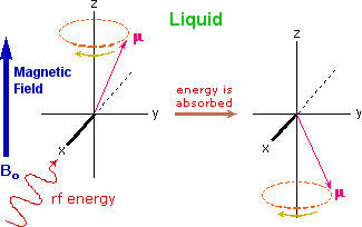
  where m is the mass, x the displacement of the object, k is the force constant for the vibrating spring, and t is the time. This equation describes exactly the case of superconducting LC-circuit if m is replaced by the inductance L, k by the inverse of the capacitance 1/C, and x by the magnetic flux (the magnetic field through an area A), i.e.,
  L d²/dt² = - /C.
- In analogy to the harmonic oscillator,
  1. The potential energy is given by the formula: U = ²/2C
  2. The flux is oscillating according to: = _max sin(2ft), where the oscillating frequency f=(1/LC)^1/2.
  3. The quantized energy levels are prescribed by E_n=(n+1/2)hf, where h is the Planck constant. Note that the spacing between adjacent levels is constant, i.e., E=hf.
  4. Since the harmonic energy levels are evenly spaced, resonant electromagnetic excitation leads to multi-photon processes that occupy excited states, and thus do not provide the clean two-level system that is needed for quantum computing. Thus a small nonlinear term must be added to the equation to product anharmonic energy levels. This requirement can be satisfied by adding the Josephson junctions to the LC-circuit (a in Figure 06a).
  5. Depending on the values of the single electron charging energy E_C=e²/2C and the Josephson energy E_J. There are three types of superconducting qubits : 1. Charge qubit with E_J/E_C<<1, inductance is omitted; 2. Flux qubit with E_J/E_C>>1, and 2 currents loop in opposite directions; 3. Phase qubit with E_J/E_C>>1, and the potential is biased at a different point (see b,e, c,g, d,h in Figure 6a).
  6. Superconductive quantum computing has the advantage that it can be supported by current technology to build the components and to have it scaled up to practical size. Figure 06b presents a simplified architecture for a superconductive quantum computer :
    - Input and output can be implemented using existing control logic in classical computers. The program in quantum computing is the sequence of gate operations that act on the qubits. This sequence is supplied by a classical computer.
    - The drivers (e.g., RF pulse) are used to control single qubits and also serve as on and off switch for inter-qubit interactions. Only couplings between adjacent qubits are depicted in the diagram.
    - The qubits are constructed as tiny LC-circuit (as mentioned above) about 0.01 to 0.0001 cm in size.
    - Couplers in the forms of superconductive circuits, electromagnetic coupling with capacitors, inductors, or microwave cavities can be used as long as they can be modulated.
    - Sensor serves as the interface between the quantum world of the qubit and classical control logic. The qubit can be coupled to a magnetometer or electrometer, and then processed by an amplifier and comparator (a device which searches for the larger one between two voltages or currents).
  Figure 06a Superconducting Qubits
  [view large image]
  
  Figure 06b Superconducting Quantum Computer
  [view large image]

Quantum computing requires entanglement between qubits. It is usually produced by sending a single photon through a certain type of crystal lattice (such as the beam splitter). The process is not very reliable until recently in June 2010, a technique has been found to generate an entangled pair of photon from a quantum dot with 82% reliability. The InAs quantum dot is embedded in a GaAs LED. When the LED is supplied with electric current, two electrons hop into two positively charged "holes" in the quantum dot's lattice, releasing a pair of entangled photon (Figure 06c). There are rooms for improvement in producing more reliable quantum dot (that can be used to generate entangled pair) and in raising the operating temperature from 5^oK.

Figure 06c Photonic Entanglement

In Figure 06c The "R" and "L" in the Bell state represent right- and left-handed circularly polarization and the first label denotes photon #1 (blue), the second label for photon #2 (green), e.g., |RL> means photon #1 in right polarization, photon #2 in left polarization.

¹An EPR-source is used to provide an entangled pair. An example is the decay of the pi meson into an electron-positron pair. Since the spin for the pi meson is 0, the spin for the electron-positron pair must be opposite according to the conservation of angular momentum. Therefore, no matter how far apart are the members of this pair, if the spin is flipped for one of the member, the spin for the other member will also be flipped to the opposite at precisely the same moment. This non-local influence (non-locality) occur instantaneously, as if some form of communication, which Einstein called a "spooky action at a distance", operates not just faster than the speed of light, but infinitely fast. Figure 04 is another method to prepare entangled pair. In this case, it is the entanglement of the horizontal and vertical polarizations of the photon. It has been demonstrated recently in 2004 that entanglement and teleportation is possible using pair of trapped ions such as Ca⁺ or Be⁺.

²To achieve projection of photon 1 and 2 into a Bell state the two photons are superposed at a beam splitter.