Quantum Field Theory

Lattice Theory

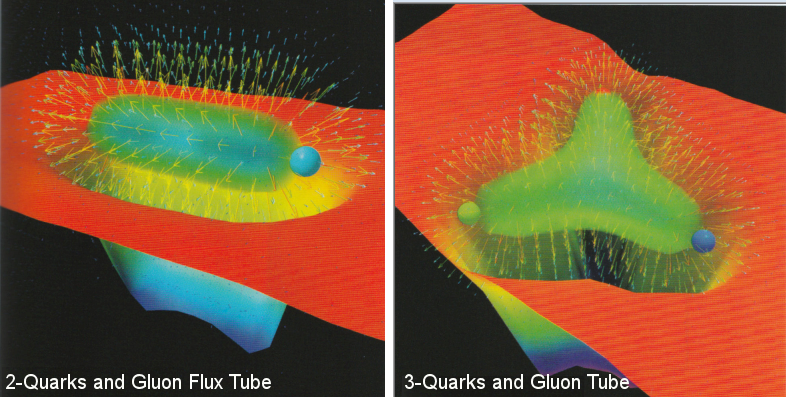
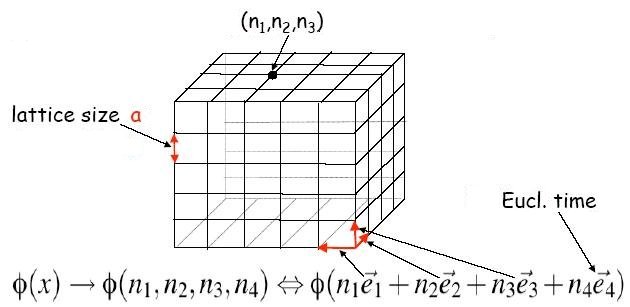
1. There are three color charges in QCD (red, green and blue), whereas QED comes with only two (the positive and negative charges). 2. The force carrier (the photon) in QED does not interact with each other, but the gluons in QCD interact among themselves. This is the reason why the photon fields spread out in QED, while the gluon fields confine to a flux tube in QCD (see Figure 05e). 3. The QCD coupling constant at large distance (~ 10-14cm) approaches to 1 making it impractical to use perturbative method. The lattice theory resorts to the use of path integral by generating thousands of paths weighted according to their likelihood under the particular rule that governs the physical evolution of the system.

Figure 05e Lattice Theory [view large image]

On the other hand, there is a price to pay for putting QCD on lattice:


1. Since the metric is Euclidean, it means that calculations with the theory are limited to the static properties of QCD such as confinement and perhaps the low-energy spectrum of states. It has difficulty calculating scattering amplitudes, which are defined in Minkowski space.
2. Lattice theory explicitly breaks continuous rotational and translational invariance, since space-time is discretized. All that is left is symmetry under discrete rotations of the lattice.
3. It is constrained by the available computational power. Many important effects (e.g., virtual pair creation etc.) are not included in the calculation back in the 20^th century.

1. The three dimensional space is discretized into a finite, periodic gird as shown in Figure 05f. 2. The fermions are located at the nodes (vertices) of the grid with link (edge) "a" in between. 3. Normal time is converted to Euclidean time, i.e., t i t. This 4th dimension will be added to the grid in Figure 05f. It follows that the transition amplitude ~ all pathseiS (where S is the action/) now changes from oscillatory to dumping form: all pathse-S.

Figure 05f 3-D Lattice [view large image]

	4. In a Feynman diagram, it would be the gauge field that goes between the fermions. However if we want to retain gauge invariant in lattice theory, the link should be identified to: U(Cxy, An) = P exp(igaCxyAnaa),
Figure 05g The Link [view large image]	where Cxy is a path between x and y (Figure 05g), P denotes path ordering, An represents the gauge field at point n, g is the coupling constant, and a are the SU(3) generators in the form of 3X3 matrices.

	5. One way to construct gauge-invariant quantities out of the links is the Wilson loop (Figure 05h), which goes around along the links in a closed path, and takes the trace (Tr) of the product from each link (trace of a matrix A: TrA = ann). It can be shown that in the continuum limit a 0, the Wilson loop reduces to a form proportional to the Yang-Mills Lagrangian.
Figure 05h Wilson Loop [view large image]	6. The Wilson action for SU(N) group can be expressed as: SW(Uij) = P[Tr(UP + UP) - 2N]

< O(U) > ~ dUijO(Uij)exp[-SW(Uij)], where denotes multiplicaltion of objects with indices i, j. In particular, the average of the Wilson loop is: < W(C) > = < Tr(U1, U2, ... Un)C > ~ exp(-TA) at the strong coupling limit, where A is the area encircled by C, and T is called the string tension. This result implies a static potential V(r) ~ Tr, where r is the separation between the quarks. Since V(r) increases with the value of r, thus it validates the concept of confinement.

Figure 05i Gluon Fields in Grid [view large image]

8. Finally, the lattice theory has to be verified that it goes over to QCD at the continuum limit as the link a 0 and the Euclidean time i t is reverted back to the normal time t. Figure 05i shows a typical pattern of activity in the gluon fields from a quark within the grid.

For the simplest possible group with only two elements, if the lattice is 8x8x8x8 in size, then the sum contains 2212 ~ 101228 terms, which is clearly prohibitive even by running all these different paths with a super computer. The Monte Carlo technique (as inspired by winning the game), however, evades this problem by the statistical sampling method wherein it does some random sampling first in order to discover the algorithms that would yield the best fit. The first result from lattice calculation was published by K. G. Wilson in 1974, who set up the Wilson loop to perform the computation in the strong-coupling limit for quark confinement as shown in Figure 05ja. The latest effort has derived a 'u' mass of 1.9 Mev and a 'd' mass of 4.4 Mev. Thus the uud quarks in a proton weigh 8.2 Mev, which is only about 1% of the proton's measured mass (938 Mev). All the rest of the proton mass comes from the energy that binds

Figure 05ja Confinement [view large image]

the quarks together. It reveals that not only the atoms are mostly empty space; now we know the nuclei inside atoms are also mere puffballs with almost no solid substance.

	In Figure 05ja, all the gluon fields are concentrated in a "flux tube" as an anti-quark is added nearby to cancel the fluctuations shown in Figure 05i. Another lattice QCD calculation from GlueX at Jefferson Lab shows the "flux tube" configurations for 2 quarks and 3 quarks respectively (Figure 05jb). The "hairs" (or arrows) are the color field lines originated from the gluons.
Figure 05jb Flux Tubes [view large image]

		QCDOC (QCD On Chip), is a series of computers designed specifically for lattice QCD calculations and dedicated more or less exclusively to that task. The glass-fronted cabinets in Figure 05k, at Brookhaven National Laboratory, hold two QCDOC machines, each with 12288 processors; a third QCDOC is at the University of Edinburgh. A typical lattice has 32 nodes along each of the three spatial dimensions and 128 nodes along the time dimension. That's about 4 million nodes altogether, and 16 million links between nodes. Some lattice
Figure 05k QCDOC [view large image]	Figure 05l Lattice	QCD simulations are run on "commodity clusters" - machines assembled out of hundreds or thousands of off-the-shelf computers. Figure 05l is an artist's imagination about the Lattice Theory - blending rows of computers with the nucleons and its quarks within.

The results (filled circles) are in remarkable agreement with the experimental values (horizontal lines). Each symbol (, K and so on) refers to a different type of hadron. The widths of the bands indicate the experimental decay widths, the invert of which are related to the finite lifetime of the particles. The vertical error bars denote the theoretical error estimates. Three of the hadrons (, K and ) have no error bars because they are used to fix the theory's parameters. Since there are (3x3x4) + (8x6) = 84 numbers at each node (quark fields have three flavours, three colours, and four components accounting for spin and antiparticles; gluon fields have eight internal directions in its symmetry group, and for each direction there are six fields: three electric and three magnetic) no computer can handle the

Figure 05ma Masses of Hadrons [view large image]

astronomical number crunching in the lattice calculation, certain approximations are adopted to make the task manageable:

1. Lattice Size - Because of asymptotic freedom, the short-wavelength fluctuations of the fields can be replaced by Gaussian random (free) fields. Thus there is a minimum lattice size, which helps to cut down the number of links. The effects of the missing fluctuations can be computed analytically and added back in.
2. Lattice Volume - It is possible to control finite-volume errors by varying the simulated volume and making theoretically informed extrapolations.
3. Small u and d quark masses - Solutions become hard to obtain with the very small physical values of these masses. They are handled by sophisticated, theoretically informed extrapolation from simulations using larger mass values.
4. Finite computer power - Even after acceptable levels of discretization and restriction to finite volume, the space that should be surveyed in the lattice calculation is far too large for even the most powerful modern computer banks to handle. So in place of a complete survey, it is replaced by a statistical sample. This introduces errors that can be estimated by the standard techniques of statistics.

In 2015, a combined QCD/QED computation obtained a numerical for the neutron-proton mass difference (Figure 05mb). The inclusion of electromagnetic interactions render further complication for the computation. In addition, the QED self-energy would be infinity. The workaround is to take the average from various combinations of quarks and eventually obtained a mass difference about 20% of the measurement of (n - p) = 1.4 Mev. It is said that such mass difference is crucial to our existence. If the proton mass is greater than the neutron's, then there would not be any protons left to make the atomic nuclei as all of them would decay to neutrons. On the other hand, if the the neutron mass is much greater than the proton's, then there would be barrier to prevent adding neutrons to form complex nuclei. The final result is published in Science (vol 347, p1452) under the title : "Ab initio calculation of the neutron-proton mass difference".

Figure 05mb n-p Mass Difference [view large image]

	The numerical calculations were performed with two IBM Blue Gene supercomputers. Figure 05mc shows the specifications. Some of the acronyms are explained below : FLOPS - Floating-point Operations Per Second. GFs - Giga FLOPS. DDR - Double Data Rate RAM. MTBF - Mean Time Before Failure. W - Watts.
Figure 05mc IBM Blue Gene Supercomputer

Go to Next Section
 or to Top of Page to Select
 or to Main Menu