
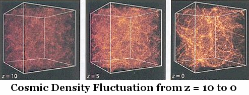
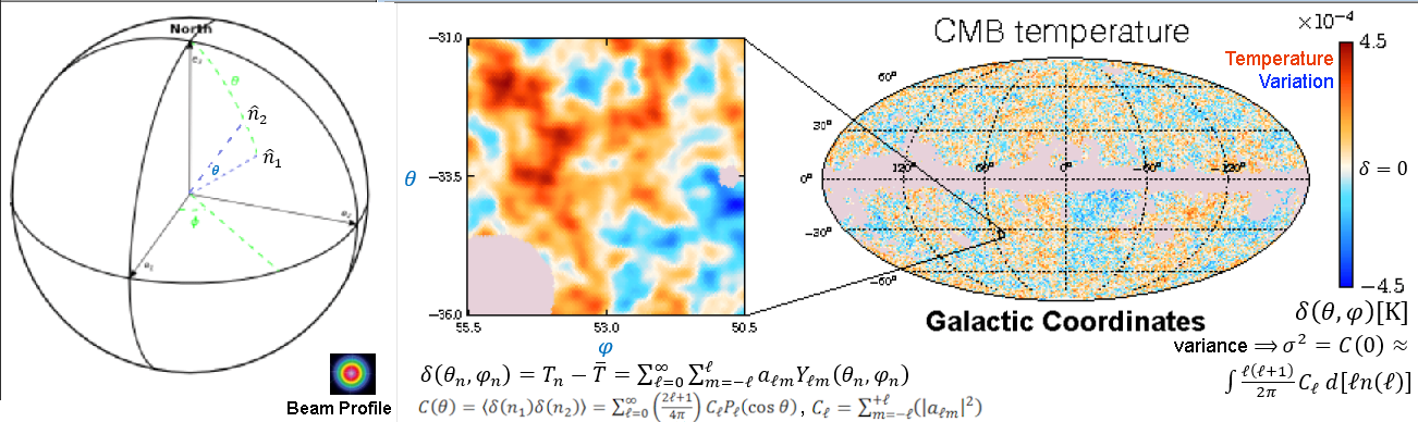
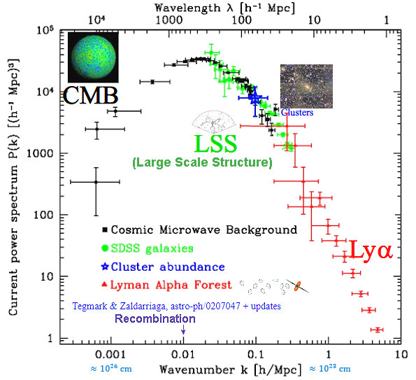
It covers 2 different cosmic structures, namely, the CMB (Cosmic Microwave Background) and CDF (Cosmic Density Fluctuation). They may look different, but basically from the same "Quantum Fluctuations" at the very beginning of the Universe. Their theoretical foundations also share the same kind of formalism.
 K. It is plotted in

 . The corresponding formula for the 2-point correlation function in
  . The C
 (k) is the amplitude and
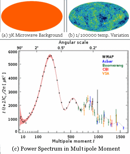
 (r). See
 (x,y) or
  /
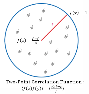
/ ) of the two-point correlation function with r = 0 (or x = y) is related to the Power Spectrum. Following is a brief sketch of the mathematics involved. BTW, the formulas become simpler in cosmology, which assumes an isotopic (rotational invariance) and homogeneous (translational invariance) mass-energy distribution so that the formulas depend only on the distance r and the absolute value of k, i.e., k = |k|.


 as an indicator for fluctuation, uncertainty, spread, ... of the measurements on certain variable x,
where
as an indicator for fluctuation, uncertainty, spread, ... of the measurements on certain variable x,
where  is the mean (average) value, and N the total number of measurements. See a graphic illustration in Figure 03a in which f(x)dx = (ni/N)dx where ni is the number of measurements within the range dx at xi.
 (x) = [d(x) - d0] / d0, where d0 is the average value. Then the correlation
  , the temperature T, or the gravitational potential
  . For the cases of


 CMB discovery via 1% of the TV static, circa 1964.
 /
/ ,
,  and a 1080p HD TV screen shot

 ).
).


 = sp then it is "believed" that the noise nt would take the role of variance
  . However, since the noise is random, it has to be treated as part of the data such that


 2Y
2Y

 (p) + e-(q)

 is the dominant factor for the collison effect on the r-h-s of
 =
=  = constant is conserved or


 k,
k,  ,
,  cd,
cd, 


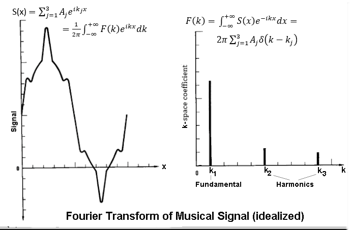
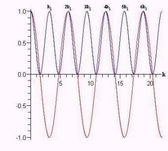
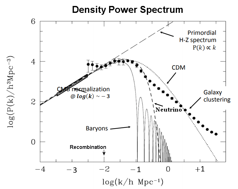
 k{Gk cos(kx)} ---------- (1)


 ), where


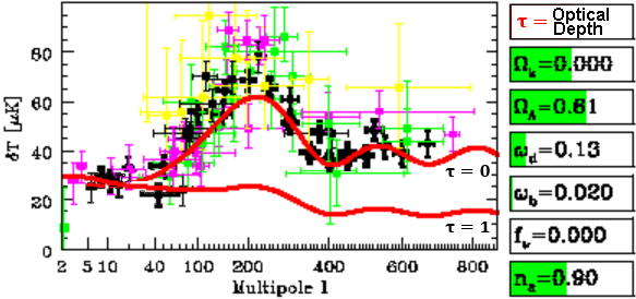
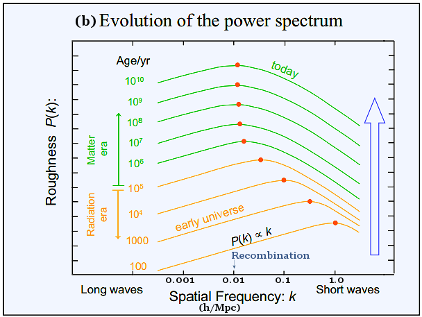
 3.6 corresponds to an age of the universe T = 1/H0 = 13.5x10⁹ years.

 is a reference-density. For example, the

 .
.
 1
1 

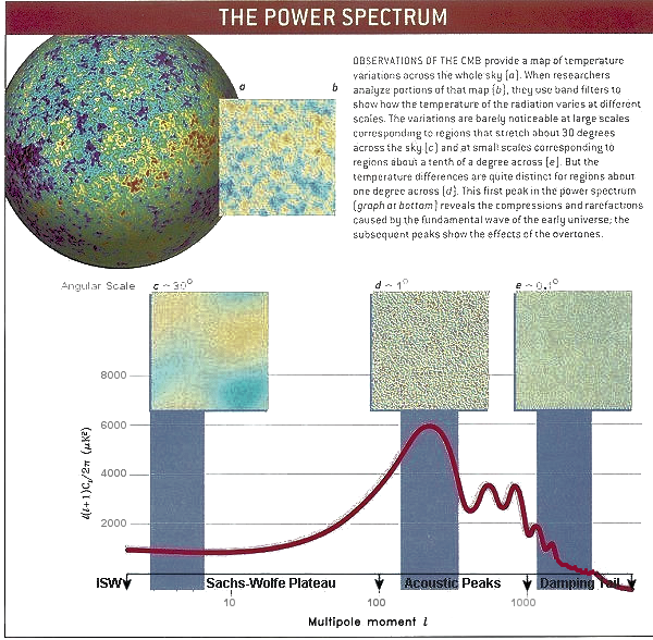
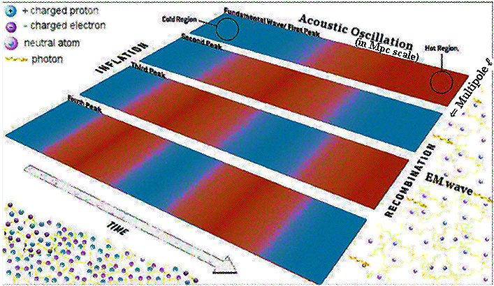
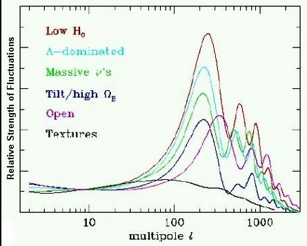
 ) in the early universe seeded density fluctuations (??), leading to temperature fluctuations (?T).
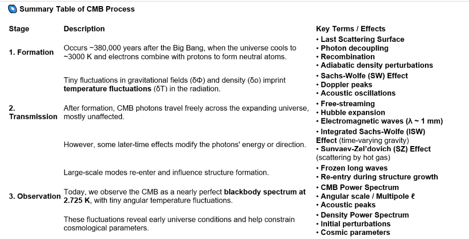

![[view large image]](I02-20-Cosmic.png)